9 Clustering
9.1 Goals
- Define groups of cells with similar transcriptional profiles, that represent the celltypes in our experiment
9.2 Overview
For an analysis, we will want to be able to examine different cell types or cell states in our data. Sadly the cells don’t come labelled, and ‘celltypes’ aren’t firm classifications anyway! But we can group together cells with similar expression profiles into ‘clusters’, which we can analyse.
9.3 Generate Clusters
To generate clusters, we first build a ‘neighbourhood’ graph. This is a network graph, that links up cells on the basis of their transcriptional similarity (‘neighbours’). Its not something for looking at directly, its simply stored inside the object, but its an important input for downstream steps like clustering.
Forget to run it and you’ll generate an error.
Note that we need to specify the ‘harmony’ reduction, else it would default to ‘pca’. Just like the UMAP, we want our clusters to represent different cell types or states, not the differences between individuals.
so <- FindNeighbors(so, reduction = "harmony", dims = 1:15)Now clustering can be as simple as running ‘FindClusters’.
# Resolution generally between 0.1 and 1
so <- FindClusters(so, resolution = 0.2 )  # A low resolution, fewer clusters
## Modularity Optimizer version 1.3.0 by Ludo Waltman and Nees Jan van Eck
##
## Number of nodes: 56853
## Number of edges: 1325795
##
## Running Louvain algorithm...
## Maximum modularity in 10 random starts: 0.9016
## Number of communities: 6
## Elapsed time: 12 seconds
so <- FindClusters(so, resolution = 1.0 ) # high res for more## Modularity Optimizer version 1.3.0 by Ludo Waltman and Nees Jan van Eck
##
## Number of nodes: 56853
## Number of edges: 1325795
##
## Running Louvain algorithm...
## Maximum modularity in 10 random starts: 0.8021
## Number of communities: 14
## Elapsed time: 12 seconds
so <- FindClusters(so, resolution = 0.8 ) # the default resolution ## Modularity Optimizer version 1.3.0 by Ludo Waltman and Nees Jan van Eck
##
## Number of nodes: 56853
## Number of edges: 1325795
##
## Running Louvain algorithm...
## Maximum modularity in 10 random starts: 0.8206
## Number of communities: 12
## Elapsed time: 12 seconds
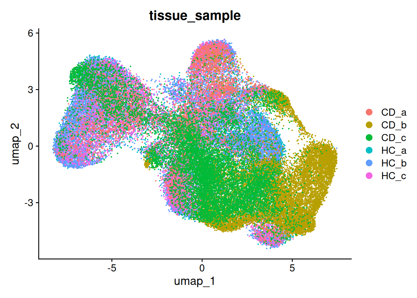
DimPlot(so, group.by='RNA_snn_res.0.2')
DimPlot(so, group.by='RNA_snn_res.0.8')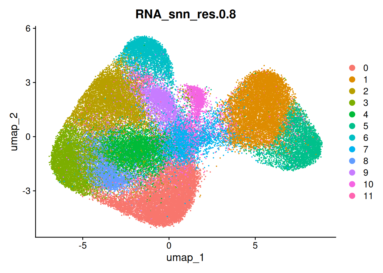
DimPlot(so, group.by='RNA_snn_res.1')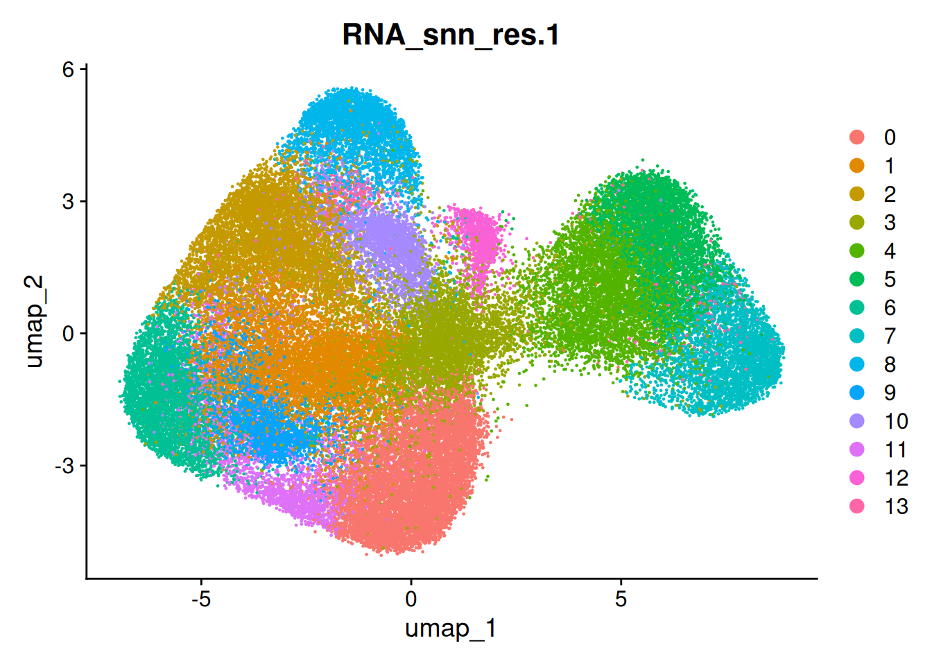
The clustree package can be a useful tool to evaluate different levels of clustering. There is an example of its use here in the context of single cell transcriptomics.
ACTIVITY What clustering resolution should we choose?
- Try another clustering resolution
- Plot it on the UMAP, and/or another clustree.
Share your results in the slack.
In real life, choosing a clustering resolution can be a cyclic process with cell type labelling. The ‘correct’ level of clustering is one that lets you answer the biological questions you are interested in. To broad and you’ll have heterogeneity in your clusters, or too specific and and you’ll have somewhat arbitrary clusters with too few cells to test anything. You may need to use different levels of clustering for different analyses, or choose to make sub-clusters in one particular celltype of interest.
For the rest of the workshop, we’ll use stick with that resolution of 0.8 - which was actually the default. Because we ran that one last, it is stored in ‘seurat_clusters’
so <- FindClusters(so, resolution = 0.8) # Rerun if you've been trying other resolutions
DimPlot(so, group.by='seurat_clusters')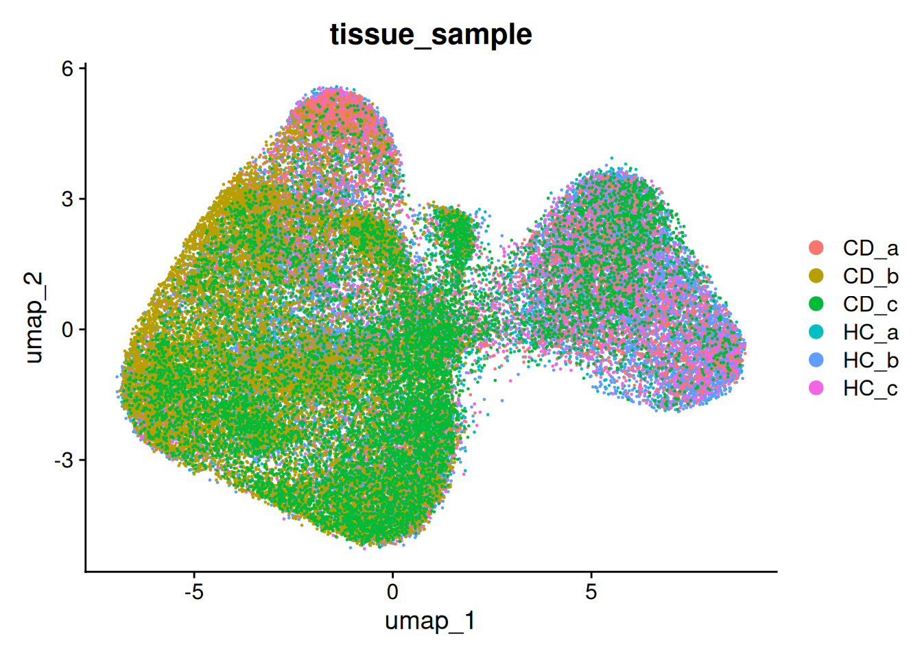
What does it look like on the tissue? Our clusters are based purely on transcriptional profiles.
so_sample <- so[, so$tissue_sample=="HC_a"]
ImageDimPlot(so_sample,
             fov          = "GSM7473682.HC.a",
             axes = TRUE,
             border.color = NA, border.size = 0.1,
             cols = 'polychrome',
             group.by = "seurat_clusters",
             boundaries   = "segmentation",
             crop=TRUE)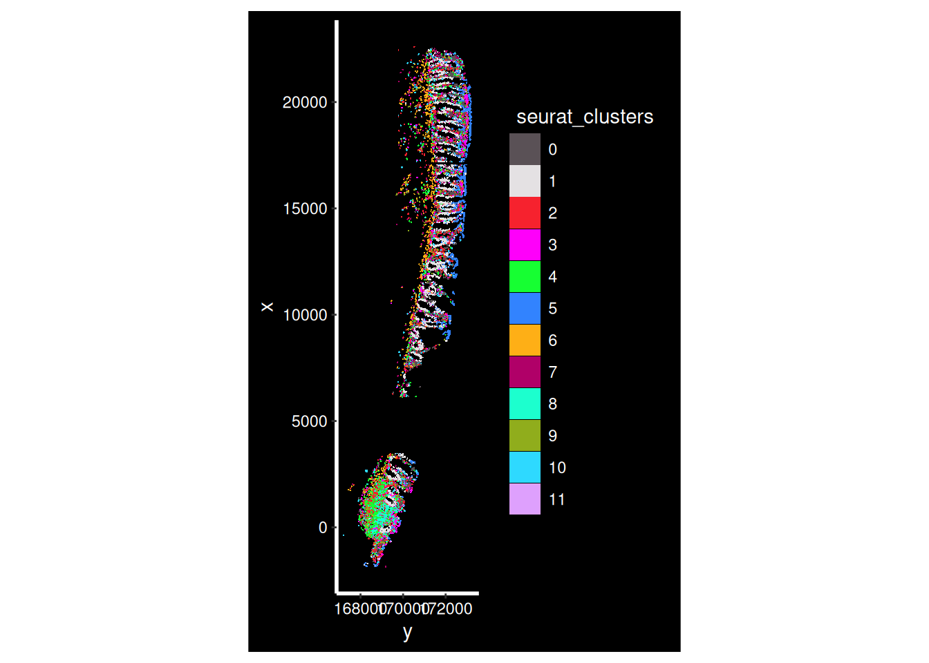
And check that our clusters are balanced across samples. What is happening with CD_b?
## Celltype proportions
celltype_summary_table<- so@meta.data %>% as_tibble() %>%
  group_by(condition, tissue_sample, seurat_clusters ) %>%
  summarise(n_cells = n())


ggplot(celltype_summary_table, aes(x=tissue_sample, y=n_cells, fill=seurat_clusters)) +
  geom_bar(position="fill", stat="identity") +
  theme_bw() +
  coord_flip() +
  theme(legend.position = "bottom") +
  scale_y_continuous(expand = c(0,0)) +
  ggtitle( "Celltype composition") +
  facet_wrap(~condition, ncol = 1, scales = 'free_y')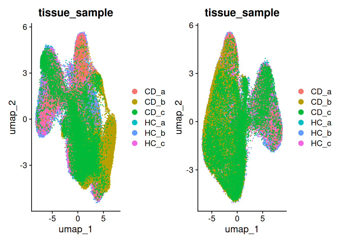
Spatially aware clustering methods
Here we are using method based purely on each cells transcriptome. You may perfer to investigate the use of a spatially-aware clustering tool such as semanticST or others (a rapidly progressing feild).