11 Spatially Restricted Genes
11.1 Goals
- Find genes that have a particularly non-random distribution (high autocorrelation) across the tissue
- Investigate what might be the reason behind the high autocorrlation of one of those genes.
11.2 Overview
What genes have a spatially restricted expression across the tissue? These might be localised to a particular region and indicate some spatial activity.
We can calculate ‘spatial autocorrelation’ with the MoransI test to find them.
11.3 Run MoransI once
To run this quickly, going to arbitrarily reduce the number of variable features to just 15. In real life, we might pick all our VariableFeatures.
so <- FindVariableFeatures(so, nfeatures=15)First lets run it for a single sample by subsetting the object.
the_sample <- 'CD_a'
the_fov    <- 'GSM7473688.CD.a'
so_sample  <- subset(so, tissue_sample == the_sample)
There’s a current bug (see ticket) with the FindSpatiallyVariableFeatures function with this kind of data. We should be able to run it directly on the seurat object itself, but as a workaround, we will run it on the ‘RNA’ assay.
# If the Seurat method above crashes (segfault), a workaround is
# running FindSpatiallyVariableFeatures at the assay level
so_sample_assay <- so_sample[['RNA']]
tc <- GetTissueCoordinates(so_sample)
rownames(tc)<- tc$cell # the innards of findSpatiallyVariableFeatures expect rownames, but they're not there. Add them.

# When given an 'assay' FindSpatiallyVariableFeatures returns an assay. Put it back in the seurat object
so_sample[['RNA']] <- FindSpatiallyVariableFeatures(
  so_sample_assay,
  layer = "scale.data",
  spatial.location = tc, # now with rownnames
  features = VariableFeatures(so_sample)[1:15], # Just a few for testing
  selection.method = "moransi",
  nfeatures=10 # mark top 10 spatially variable
)
The results end up in the gene level metadata. Pull them out, but only display the genes we ran.
#Put feature name as a column in the feature metadata
so_sample[["RNA"]]@meta.data$feature <-rownames(so_sample[["RNA"]])
gene_metadata <- so_sample[["RNA"]]@meta.data

gene_metadata_morans <-
  filter(gene_metadata, !is.na(moransi.spatially.variable.rank)) %>%
  select(feature,
         MoransI_observed, MoransI_p.value, moransi.spatially.variable,moransi.spatially.variable.rank) %>%
  arrange(moransi.spatially.variable.rank)

DT::datatable(gene_metadata_morans, width = '100%')
What do some of these genes look like on the tissue? How can we interpret this?
ImageDimPlot(so_sample,
             molecules = 'IGHA1',
             group.by = 'tissue_sample', cols = c("grey30"), # Make all cells grey.
             boundaries = "segmentation",
             border.color = NA, axes = T, crop=TRUE) + ggtitle(the_sample)
ImageDimPlot(so_sample,
             molecules = 'AQP8',
             group.by = 'tissue_sample', cols = c("grey30"), # Make all cells grey.
             boundaries = "segmentation",
             border.color = NA, axes = T, crop=TRUE)+ ggtitle(the_sample)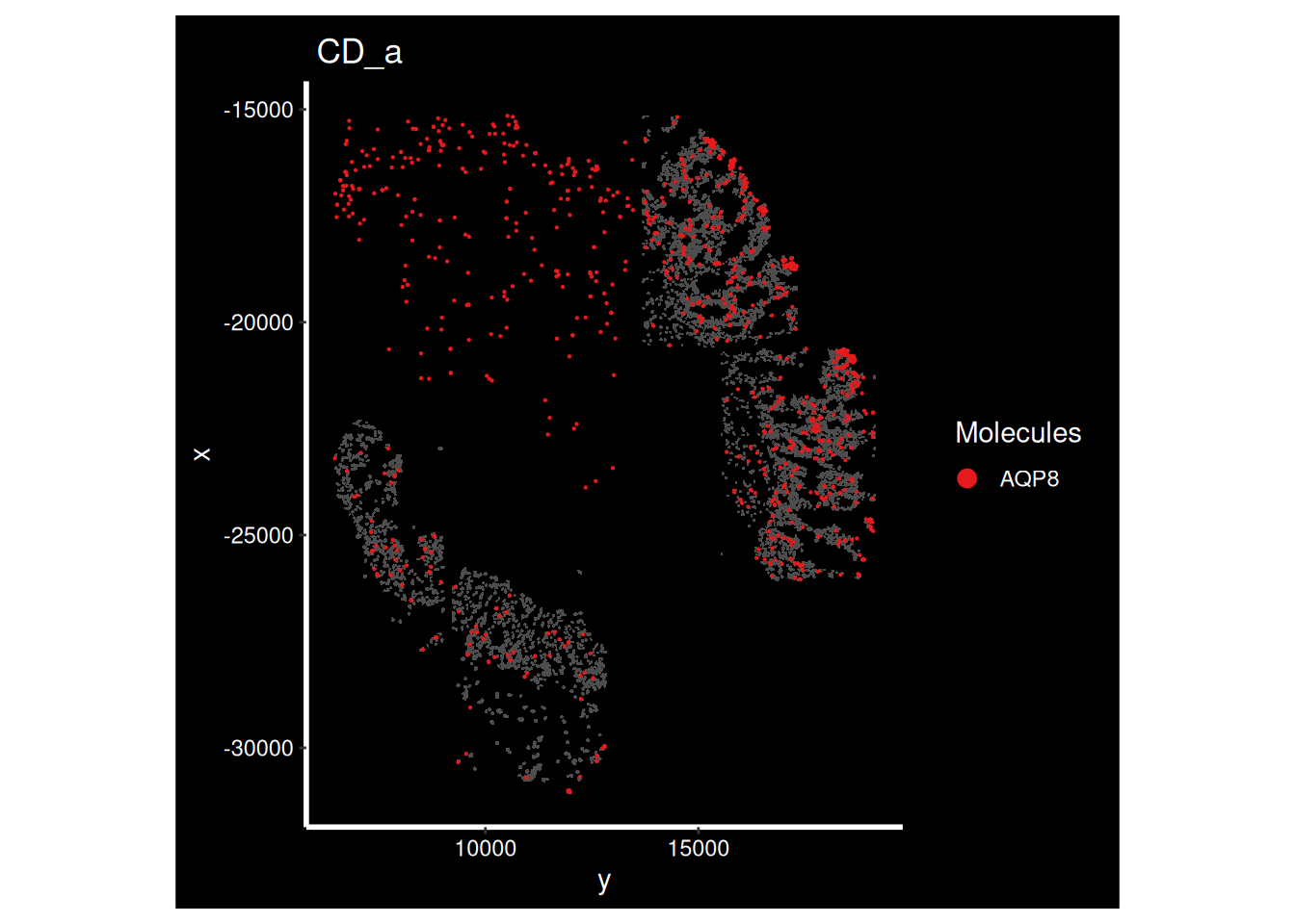
ImageDimPlot(so_sample,
             molecules = 'KRT20',
             group.by = 'tissue_sample', cols = c("grey30"), # Make all cells grey.
             boundaries = "segmentation",
             border.color = NA, axes = T, crop=TRUE)+ ggtitle(the_sample)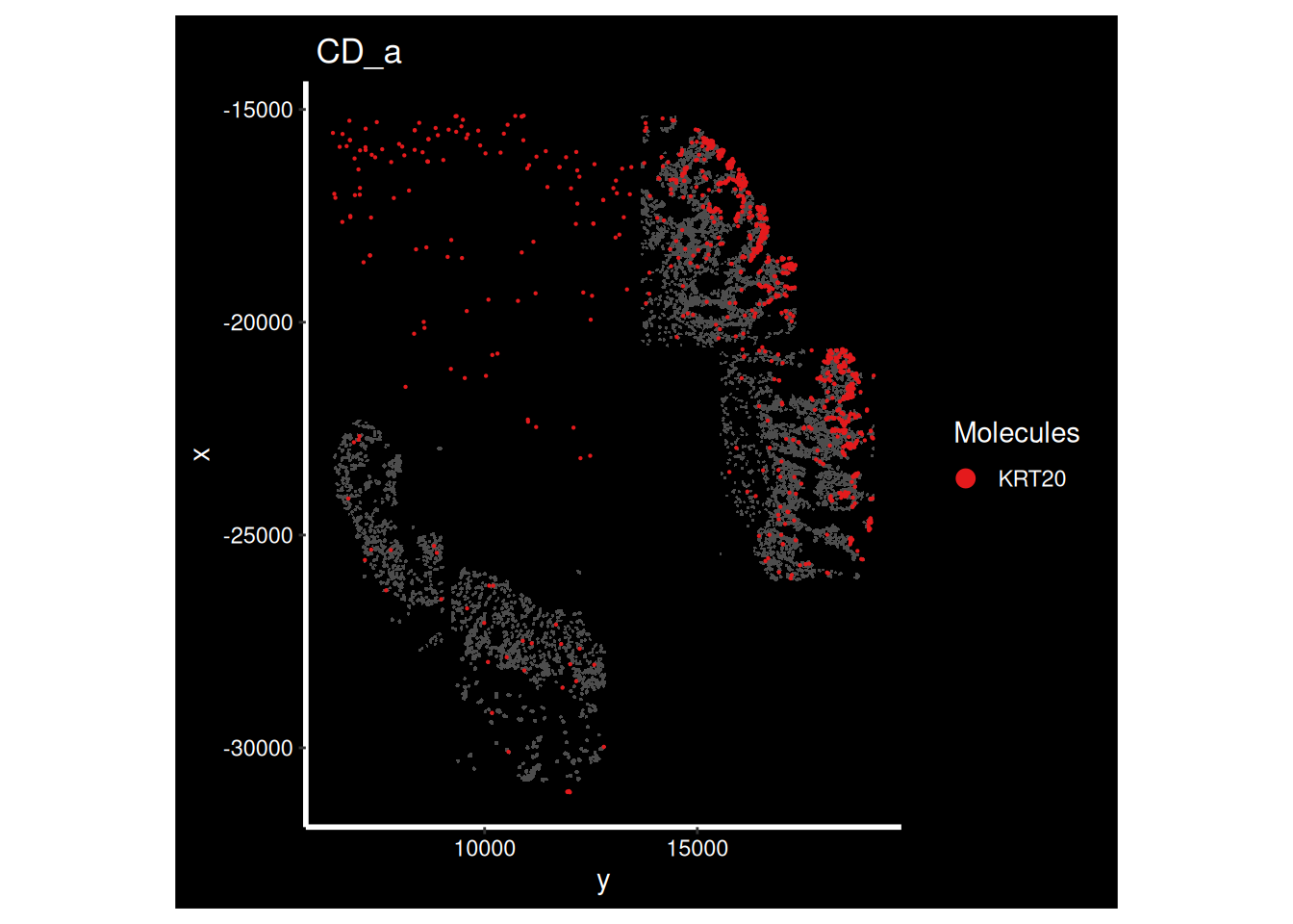
11.4 Run MoransI on all samples
Could it be that the expression pattern of a gene is disrupted? Is there a difference between samples or between groups?
Lets run the test on every sample. This is slow - do not run on the workshop machines, instead load the precomputed results.
For real life, it could be parallelised and/or run overnight.
## Do Not Run ##

# Record moransI results for each sample, one by one.
samples <- unique(so@meta.data$tissue_sample)
results_list <- list()
for (the_sample in samples) {

  so.sample <- subset( so, subset= tissue_sample == the_sample)

  so.sample.assay <- so.sample[['RNA']]
  tc <- GetTissueCoordinates(so.sample)
  rownames(tc)<- tc$cell
  # When given an 'assay' FindSpatiallyVariableFeatures returns an assay. Put it back in the seurat object.
  so.sample[['RNA']] <- FindSpatiallyVariableFeatures(
    so.sample.assay,
    layer = "scale.data",
    spatial.location = tc,
    features = VariableFeatures(so.sample),
    selection.method = "moransi",
    nfeatures=15 # mark top 10 spatially variable
    )
  # --- end workaround


  # Format output table
  so.sample[["RNA"]]@meta.data$feature <- rownames(so.sample[["RNA"]])
  gene_metadata <- so.sample[["RNA"]]@meta.data
  results <-
  select(gene_metadata,
         feature,
         MoransI_observed,
         MoransI_p.value,
         moransi.spatially.variable,
         moransi.spatially.variable.rank) %>%
    filter(!is.na(moransi.spatially.variable.rank)) %>% # only tested
    arrange(moransi.spatially.variable.rank) %>%
    mutate(sample = the_sample) %>%
    select(sample, everything())


  results_list[[the_sample]] <- results
}

# Collect output result
results_all <- bind_rows(results_list)


# Add group by deleting pulling out the sample name with everything after _ deleted.
results_all$group <- gsub("_.*","", results_all$sample)

morans_results_file <- file.path("data", "morans_results.RDS")
saveRDS(results_all, morans_results_file)
Load preprepared results file
morans_results_file <- file.path("data", "morans_results.RDS")
results_all <- readRDS(morans_results_file)
Lets visualise our MoransI scores for each gene for each sample on a boxplot. Note that this isn’t an established standard way of interpreting these scores, but it does give us a way to prioritise what to look at.
MoransI scores are between -1 (anticorrelated) and 1 (perfectly correlated) - 0 is random. The baseline isn’t 0 - probably because the observations are already limited to the tissue. But there’s still clearly some genes with higher scores than others, even though the variation between samples is quite high.
# unique set of genes that were top 10 morans in any sample
plot_genes <- filter(results_all, moransi.spatially.variable.rank <= 10) %>% pull(feature) %>% unique()
ggplot(filter(results_all, feature %in% plot_genes), aes(x=feature, y=MoransI_observed)) +
  geom_boxplot() +
  geom_point( mapping=aes(col=sample)) +
  theme_bw() +
  ggtitle("MoransI Per sample") +
  facet_wrap(~group, ncol=1)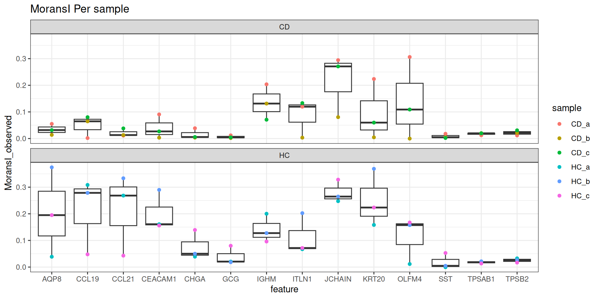
11.5 Explore moransI results
That doesn’t mean much in isolation, so lets look at the actual distribution of some of those.
so.CD_a <- subset( so, subset= tissue_sample == 'CD_a')
so.HC_a <- subset( so, subset= tissue_sample == 'HC_a')
IGHM has high autocorrelation all over
p1 <- ImageDimPlot(so.CD_a,
             molecules = 'IGHM',
             group.by = 'tissue_sample', cols = c("grey30"), # Make all cells grey.
             boundaries = "segmentation", border.color = NA, axes = T, crop=TRUE)
p2 <- ImageDimPlot(so.HC_a,
             molecules = 'IGHM',
             group.by = 'tissue_sample', cols = c("grey30"), # Make all cells grey.
             boundaries = "segmentation", border.color = NA, axes = T, crop=TRUE)
p1 + p2 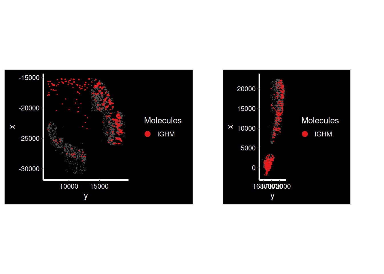
Contrast that with a CHGA - still a highly variable gene, with a low(er) spatial autocorrelation
p1 <- ImageDimPlot(so.CD_a,
             molecules = 'CHGA',
             group.by = 'tissue_sample', cols = c("grey30"), # Make all cells grey.
             boundaries = "segmentation", border.color = NA, axes = T, crop=TRUE)
p2 <- ImageDimPlot(so.HC_a,
             molecules = 'CHGA',
             group.by = 'tissue_sample', cols = c("grey30"), # Make all cells grey.
             boundaries = "segmentation", border.color = NA, axes = T, crop=TRUE)
p1 + p2 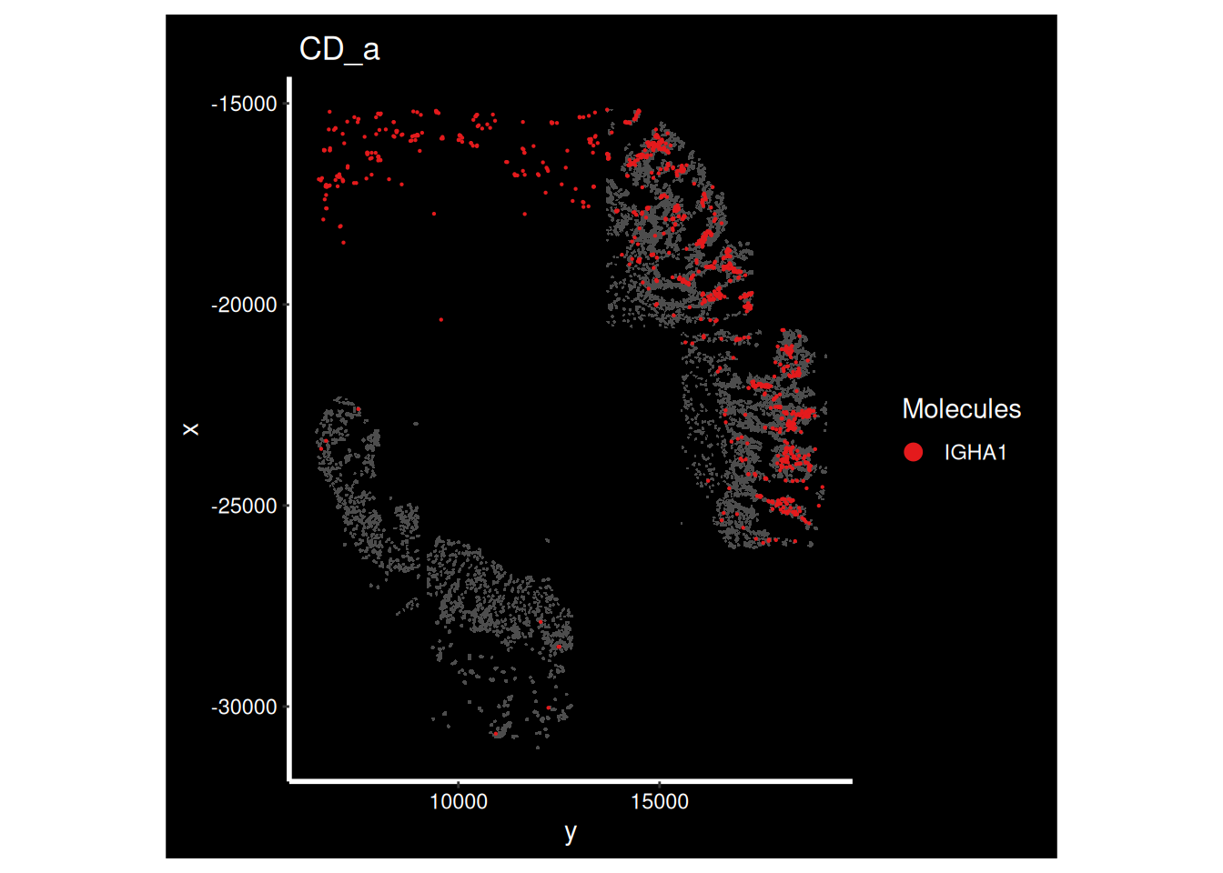
CCL21 has a combination of high and low scores. Why?
p1 <- ImageDimPlot(so.CD_a,
             molecules = 'CCL21',
             group.by = 'tissue_sample', cols = c("grey30"), # Make all cells grey.
             boundaries = "segmentation", border.color = NA, axes = T, crop=TRUE)
p2 <- ImageDimPlot(so.HC_a,
             molecules = 'CCL21',
             group.by = 'tissue_sample', cols = c("grey30"), # Make all cells grey.
             boundaries = "segmentation", border.color = NA, axes = T, crop=TRUE)
p1 + p2 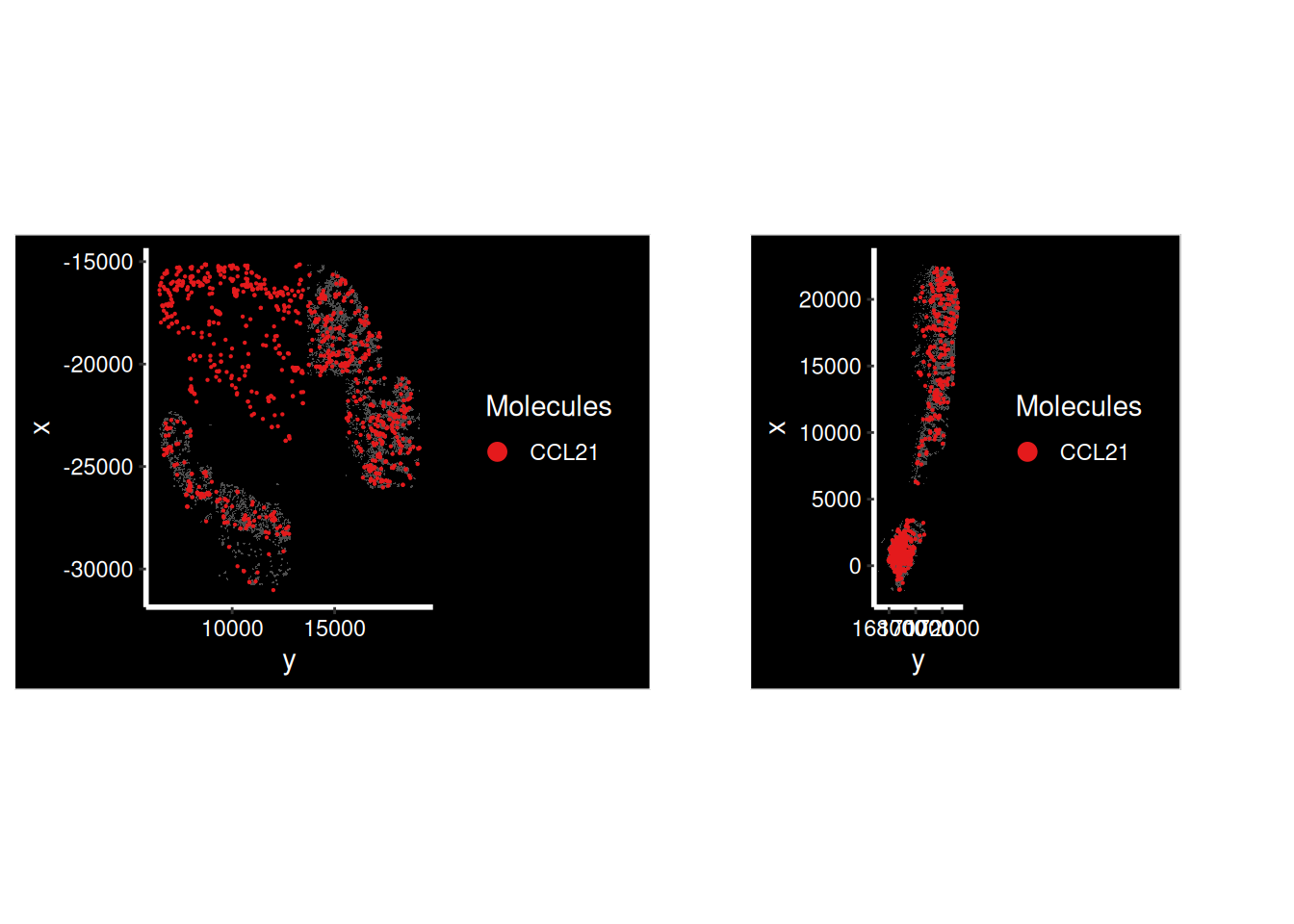
There’s a big clump of CCL21 at the bottom of HC_a, lets figure out which FOV that is and zoom in further. Now we can practically bring back the cluster labels.
ImageDimPlot(so.HC_a, group.by = 'fov')
so.HC_a.4 <- subset(so.HC_a, fov==4)

ImageDimPlot(so.HC_a.4,
             molecules  = 'CCL21',
             group.by   = 'cluster_labels', alpha=0.3,# Show clusters, but faded
             cols = 'polychrome',
boundaries = "segmentation", border.color = NA, axes = T, crop=TRUE) 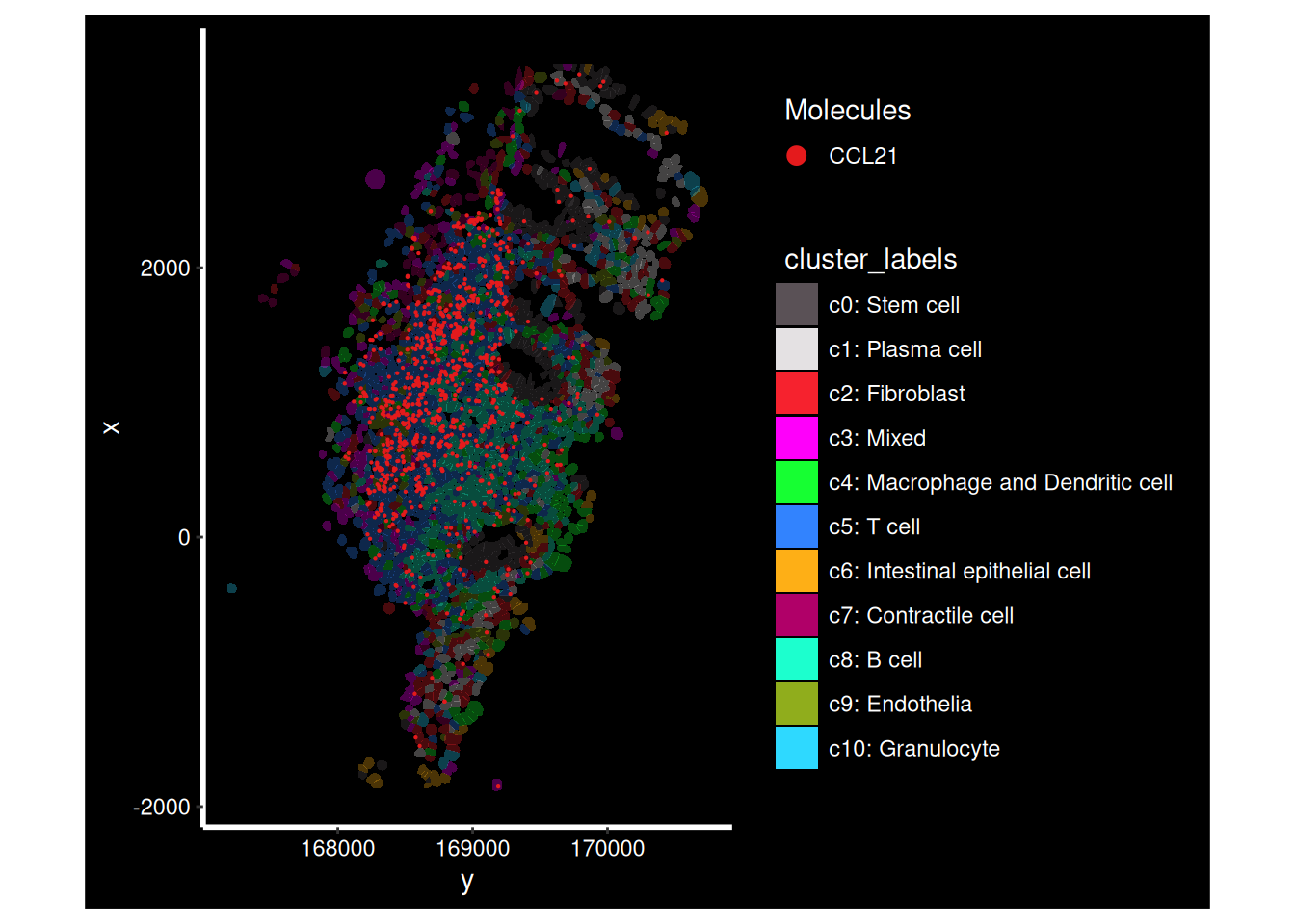
That seems to be because of a group of T cells expressing CCL21’s. We can highlight those alongside our transcripts.
# Show only B and T cells
so.HC_a.4$isBT <- ifelse(so.HC_a.4$cluster_labels %in% c("c5: T cell", "c8: B cell"), as.character(so.HC_a.4$cluster_labels), "Other")
ImageDimPlot(so.HC_a.4,
             molecules  = 'CCL21',
             group.by   = 'isBT', alpha=0.3,# Show clusters, but faded
             cols = c("c5: T cell"='royalblue', "c8: B cell"='aquamarine', 'Other'='grey80'),
boundaries = "segmentation", border.color = NA, axes = T, crop=TRUE) 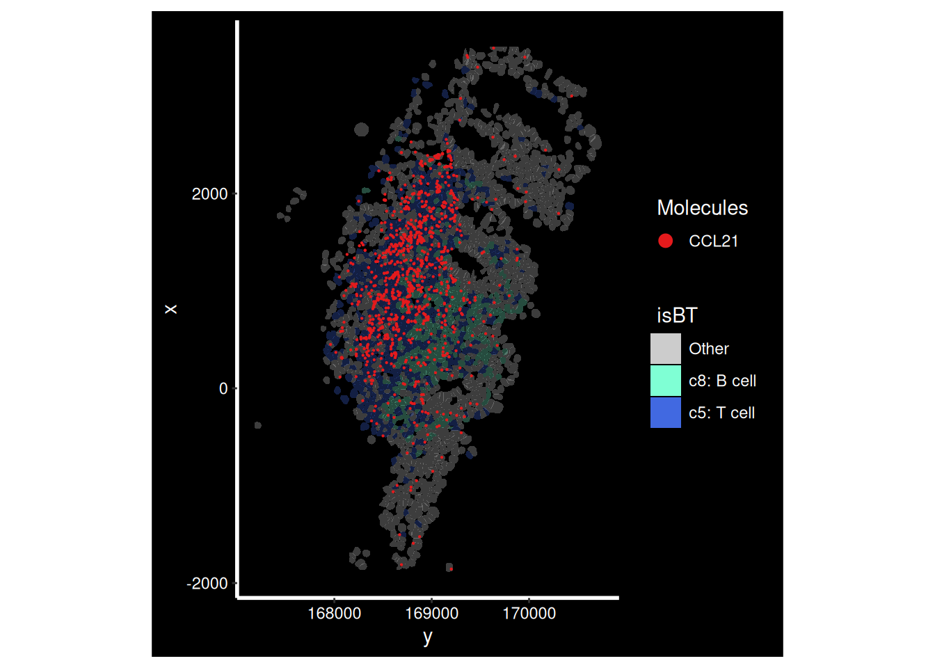
If we look at Garrido-Trigo et al’s paper - they highlight these kind of lymphoid niches, full of T, B and plasma cells. They go on to look at macrophage subtypes within these regions across different conditions.
In our case, these could be more formally defined by a niche-neighbourhood analysis; which at the most basic level, classifies each cell into a ‘niche’ depending on what type of cells are in its immediate vicinity. We could then analyse our data at the ‘niche’ level.