10 Clustering Labeling
10.1 Goals
- Evaluate what type of cell might be in each cluster using multiple lines of evidence:
- Genes that are expressed specifically in the cluster
- Find a public dataset of colon samples, and use a ‘cell typing’ tool to classify cells according to its categories
- Location of clusters within tissue
- Discuss value of histology images
- Make an informed choice on a celltype label for each cluster, and it for downstream analysis.
10.2 Overview
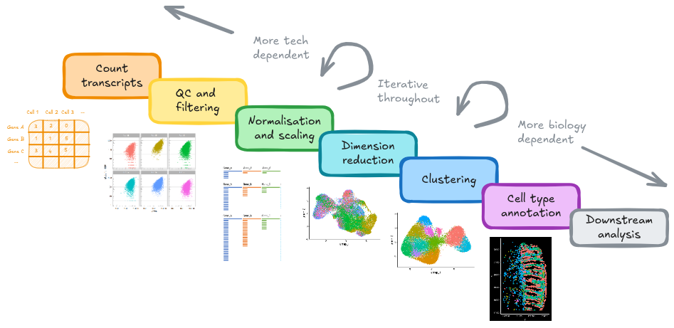
Classifying cells into meaningful celltypes (or cell states) is a time consuming, but extremely important, part of a spatial analysis.
It may involve pulling together multiple lines of evidence to assign celltype labels to cluster labels. Some approaches outlined below:
10.3 Cluster Markers
Considering our clusters - lets find some more meaningful labels than 1-10! What genes are expresses specifically in each of these clusters?
DimPlot(so, group.by='seurat_clusters')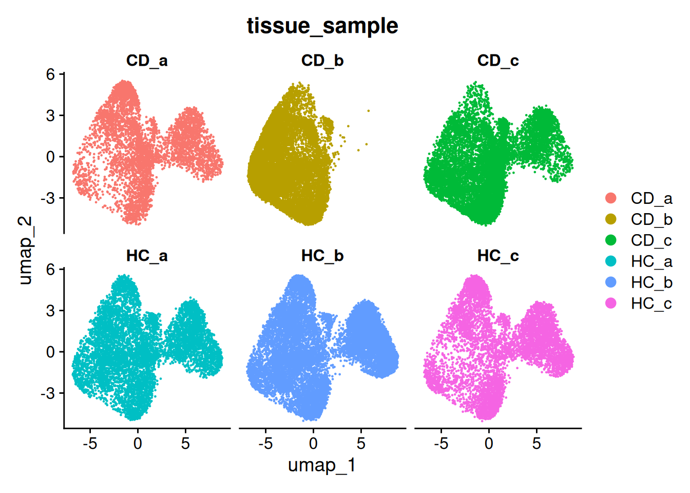
The ‘FindAllMarkers’ function runs a differential expression test to see what genes are expressed differently between each celltype and the rest of the experiment. The ‘only.pos’ parameter is useful to report only genes enriched (not absent) in each cluster.
# Need to join the layers back again for this.
so <- JoinLayers(so)
marker_table <- FindAllMarkers(so, group.by='seurat_clusters', only.pos=TRUE)
Now we have a list of ‘marker’ genes. They’re not markers in the sense of canonical celltype markers - they’re just defined from the data.
- Look at those p-values! They’re extremely significant because each cell is treated as a replicate (and samples are ignored).
- We can filter on fold-change (avg_log2FC) of expression to emphasise more interesting larger change (as even very small difference can be significant, but not useful for determining cell types).
The human protein atlas is a useful site to look up the single cell RNA expression of a given gene; e.g. CD37
DT::datatable(marker_table)A dot plot is a convenient way to summarise the top few distinct genes. It can let you read off some obvious celltypes and see similarities between clusters.
# Get top 3 genes per cluster, with log FC > 1
marker_table_top <- marker_table %>%
    group_by(cluster) %>%
    dplyr::filter(avg_log2FC > 1, p_val_adj < 0.01) %>%
    slice_head(n = 3)

DotPlot(so, features = unique(marker_table_top$gene)) + theme(axis.text.x = element_text(angle = 90, vjust = 0.5, hjust=1))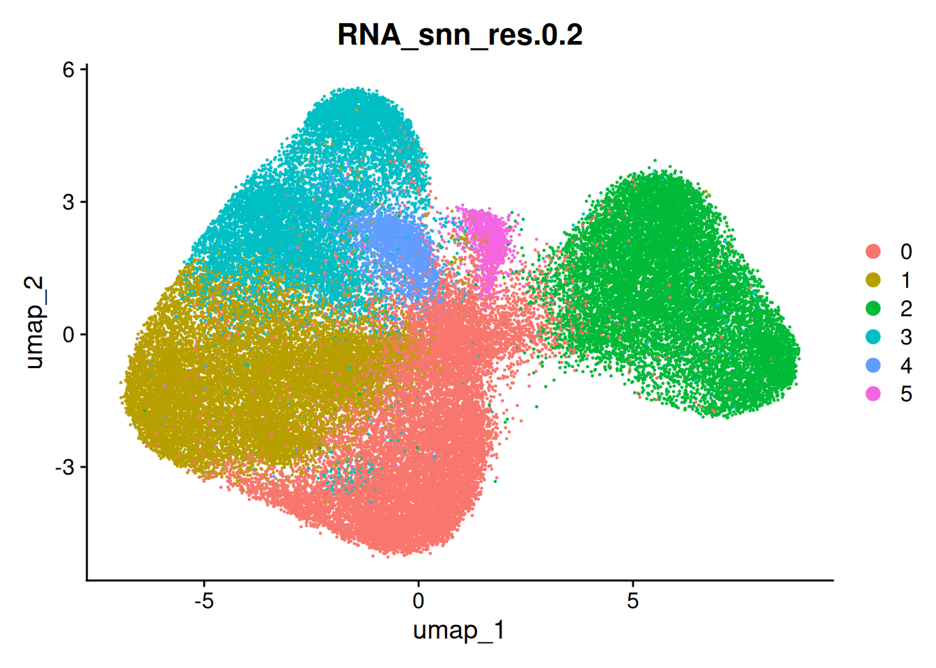
You can get some more information form these marker lists by dropping them into a tool like enrichr and considering cell type enrichment. NB: enrichR also has a R package, and could be done programatically
top_marker_genes <- filter(marker_table, cluster == "1") %>% dplyr::filter(avg_log2FC > 1, p_val_adj < 0.01) %>% pull(gene) %>% head(20)
print(noquote(top_marker_genes))
## [1] PIGR EPCAM KRT8 FCGBP KRT19 AGR2 LGALS3 ITLN1 CLDN4 CD9
## [11] S100A6 KRT18 SOX9 CD24 DDR1 CDH1 LGALS9 OLFM4 GSTP1 APP10.4 Cell typing by reference
There are a number of tools that classify cells into types on the basis of similarity with a reference dataset. SingleR is one such tool.
But first we need to acquire a reference dataset.
A typical reference would be from a public single cell datasets from a matched celltype with a trusted annotation. Look for a relevant paper which has provided their GEO accession number or similar. Note that not every study remembers to publish their annotations alongside their raw data, but the authors might be willing to supply you with a processed dataset if you ask.
Alternatively, there are some databases of single cell datasets - see Human Cell Atlas or CELLxGENE datasets. These databases also let you browse the data online - which is an excellent resource for the design or cell annotation stages; you can look up gene expression in a particular celltype to see if it matches what you are seeing.
The tabula sapiens project (paper) as built a single cell atlas from a good number of human tissues. Its data is browse-able and hosted in the cellXgene tabular sapiens collection
These are colon tissue samples, and there is a large intestine set listed (which includes colon samples). Conveniently, we can browse the data online to check if it will be suitable: via a cellXgene interface
Broad cell class looks pretty good. There’s colon included. Some individual level effect in the UMAP (stem cells limited to 1-2 samples). It’ll work, and there’s an easy link to download the data.
The reference dataset has been pre-downloaded onto the VMs
# Do not run, but these were the linux shell commands to get and rename the data
wget https://datasets.cellxgene.cziscience.com/82e3b450-6704-43de-8036-af1838daa7df.h5ad
mv 82e3b450-6704-43de-8036-af1838daa7df.h5ad tabula_sapiens_large_intestine_82e3b450-6704-43de-8036-af1838daa7df.h5ad
Its a .h5ad file, common from pythonic analyses. Luckily we can use the schard package to read it into R directly. But not to a seurat object.
This code will load, subset and convert the raw data. We will not run it here.
## Do not run ##

library(schard)

ts_largeintestine_h5ad <- file.path("data/tabula_sapiens/tabula_sapiens_large_intestine_82e3b450-6704-43de-8036-af1838daa7df.h5ad")
sce.ts_intestine = schard::h5ad2sce(ts_largeintestine_h5ad)
Instead it builds a SingleCellExperiment object - a data format central to bioconductor packages (this is fine, SingleR is from bioconductor too!). SCE objects work quite similarly to seurat objects, but have different notation - e.g. colData and rowData access the cell and gene information respectively.
## Do not run ##
DT::datatable(head(as.data.frame(colData(sce.ts_intestine))))
DT::datatable(head(as.data.frame(rowData(sce.ts_intestine))))The gene names in that object are ensemble gene IDs - let change them to gene symbols to match our data.
## Do not run ##

# Not needed, but first filter down to matched genes in our panel
sce.ts_intestine.genename <- sce.ts_intestine[rowData(sce.ts_intestine)$feature_name %in% rownames(so),]

# Are there any duplicates (we'd need to handle them, but there aren't)
# takes the count of each feature, then checks that there aren't any >1
stopifnot(sum(table(rowData(sce.ts_intestine.genename)$feature_name) != 1 ) == 0)

# just rename the genes to the gene names
rownames(sce.ts_intestine.genename) <-  rowData(sce.ts_intestine.genename)$feature_name

# Pull out the normalised matrix.
# Quirk of this coming from the python world, the normalised assay is called 'X'
ref_norm_matrix <- assay(sce.ts_intestine.genename, 'X')
The following code makes celltype predictions using the reference at the broad and specific annotation levels. It takes a few minutes to run - even with 8 cores.
## Do not run ##

library(BiocParallel) # allow parallelisation with MulticoreParam().

norm_matrix <- GetAssayData(so, assay = 'RNA', layer = 'data')

predictions_broad <- SingleR::SingleR(test = norm_matrix,
                                ref   = ref_norm_matrix,
                                labels = sce.ts_intestine.genename$broad_cell_class,
                                aggr.ref = TRUE, # builds a pseudobulk reference , speedier processing
                                BPPARAM = MulticoreParam(workers=8)
                                )

predictions_detailed <- SingleR::SingleR(test = norm_matrix,
                                ref   = ref_norm_matrix,
                                labels = sce.ts_intestine.genename$cell_type,
                                aggr.ref = TRUE, # builds a pseudobulk reference , speedier processing
                                BPPARAM = MulticoreParam(workers=8)
)

# Save results to disk, for reloading during workshop
predictions_broad_file <- file.path("data","predictions_with_ts_intestine_broad_cell_class.RDS")
predictions_detailed_file <- file.path("data","predictions_with_ts_intestine_detailed_celltype.RDS")
saveRDS(predictions_broad, predictions_broad_file)
saveRDS(predictions_detailed, predictions_detailed_file)
Load the previously saved results.
predictions_broad_file    <- file.path("data","predictions_with_ts_intestine_broad_cell_class.RDS")
predictions_detailed_file <- file.path("data","predictions_with_ts_intestine_detailed_celltype.RDS")
predictions_broad    <- readRDS(predictions_broad_file)
predictions_detailed <- readRDS(predictions_detailed_file)
The predictions look like this;
predictions_broad## DataFrame with 56853 rows and 4 columns
## scores labels delta.next
## <matrix> <character> <numeric>
## HC_a_1_1 0.1252298:0.0506561:0.146099:... intestinal epithelia.. 0.1580519
## HC_a_2_1 0.1815377:0.1348928:0.249264:... intestinal epithelia.. 0.1897494
## HC_a_3_1 0.0518528:0.0279213:0.059416:... intestinal epithelia.. 0.0542868
## HC_a_4_1 0.1243137:0.1179463:0.130171:... intestinal epithelia.. 0.0472000
## HC_a_5_1 0.1256039:0.0411866:0.114864:... intestinal epithelia.. 0.0970837
## ... ... ... ...
## CD_c_2598_4 0.0904283:0.1638795:0.0945435:... lymphocyte of b line.. 0.05787367
## CD_c_2599_4 0.1015837:0.2218872:0.1498716:... lymphocyte of b line.. 0.08493387
## CD_c_2604_4 0.0225413:0.1048716:0.0181309:... lymphocyte of b line.. 0.00208670
## CD_c_2606_4 0.1538878:0.1968389:0.1524932:... lymphocyte of b line.. 0.00544398
## CD_c_2608_4 0.0128855:0.0411252:0.0319291:... innate lymphoid cell 0.00176397
## pruned.labels
## <character>
## HC_a_1_1 intestinal epithelia..
## HC_a_2_1 intestinal epithelia..
## HC_a_3_1 intestinal epithelia..
## HC_a_4_1 intestinal epithelia..
## HC_a_5_1 intestinal epithelia..
## ... ...
## CD_c_2598_4 lymphocyte of b line..
## CD_c_2599_4 lymphocyte of b line..
## CD_c_2604_4 lymphocyte of b line..
## CD_c_2606_4 lymphocyte of b line..
## CD_c_2608_4 innate lymphoid cellPull them both into the annotation
# Check that the order of cells is the same
stopifnot(all(rownames(predictions_broad) == colnames(so)))

# Then pull in the celltypes from pruned labels, and the 'delta.next' score for each.
so$singleR_pred_broad    <- predictions_broad$pruned.labels
so$singleR_pred_detailed <- predictions_detailed$pruned.labels
so$singleR_delta.next_broad    <- predictions_broad$delta.next
so$singleR_delta.next_detailed <- predictions_detailed$delta.next
And plot on the UMAP
The broad predictions
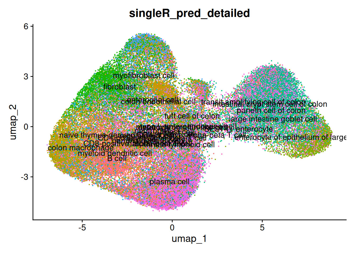
DimPlot(so, group.by = 'singleR_pred_broad', label = TRUE) 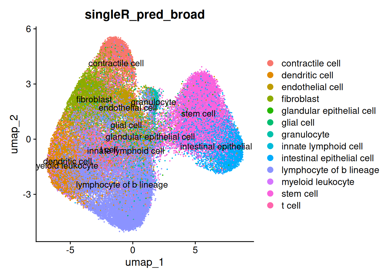
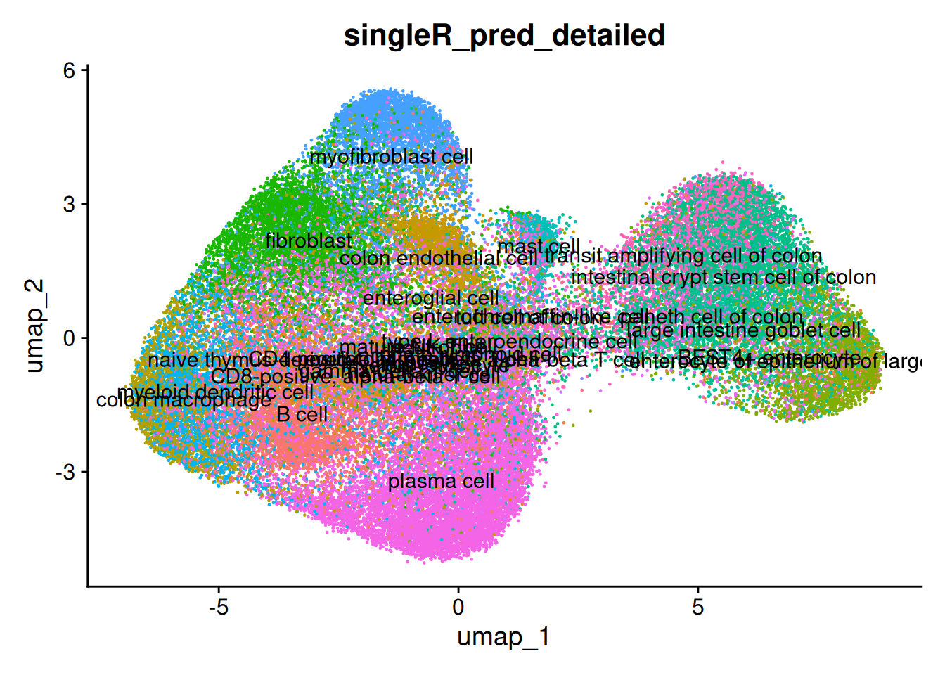
And the detailed predictions. The detailed celltypes are more difficult to see - but some have clearly labelled.
The delta next score gives you the distance between the called celltype, and the next most likely. A small difference could indicate uncertainty - from a difficult to classify cell, stray counts from a neighbouring cell or cell types that are very similar (especially in the detailed classification).
FeaturePlot(so, c('singleR_delta.next_broad','singleR_delta.next_detailed'))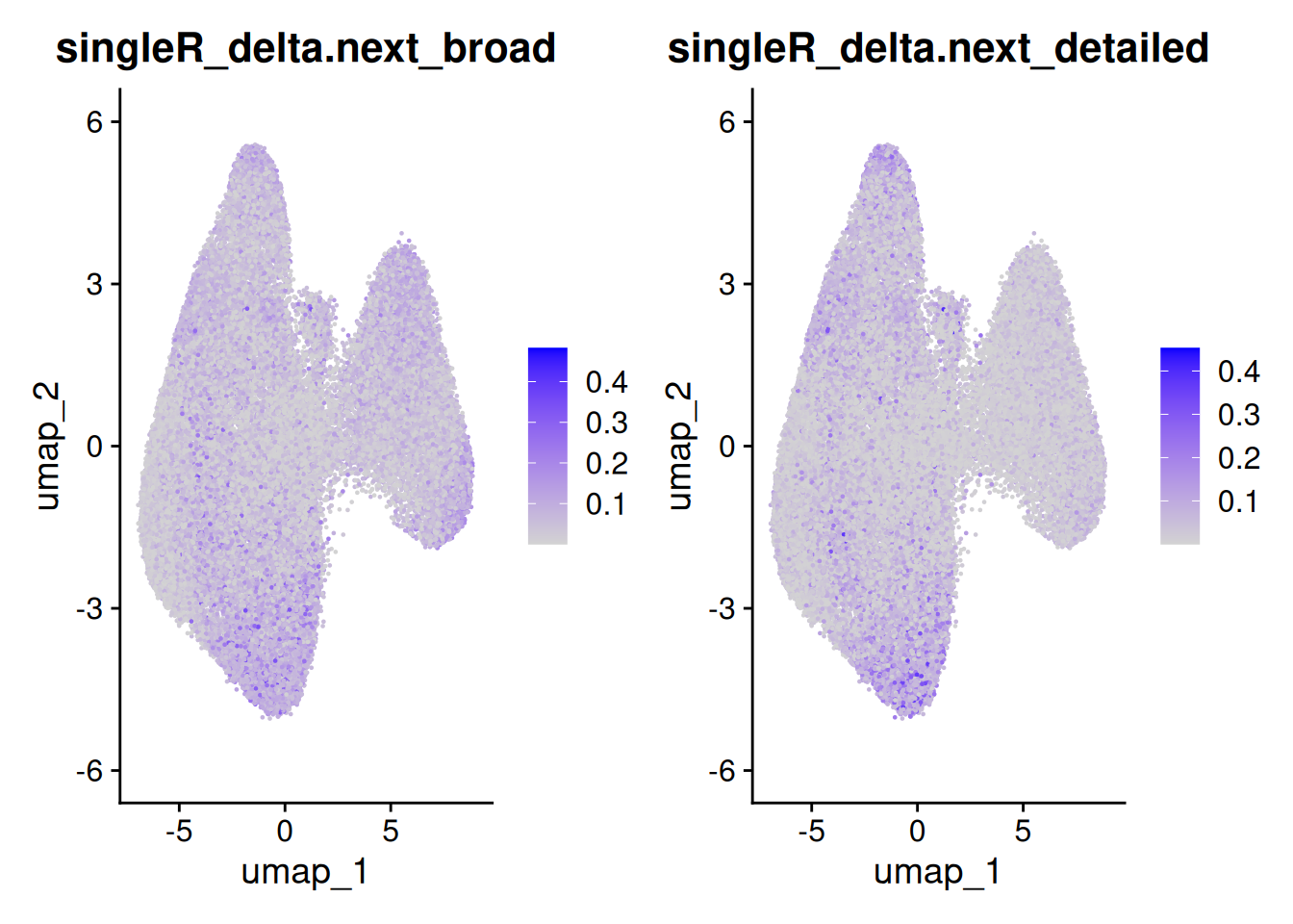
VlnPlot(so, features='singleR_delta.next_broad', group.by='singleR_pred_broad', pt.size = 0) + NoLegend()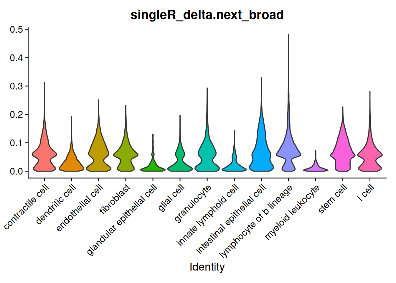
Its nice to line those classifications up with clusters.
## Celltype proportions
celltype_summary_table<- so@meta.data %>% as_tibble() %>%
  group_by(seurat_clusters, singleR_pred_broad ) %>%
  summarise(n_cells = n())


ggplot(celltype_summary_table, aes(x=seurat_clusters, y=n_cells, fill=singleR_pred_broad)) +
  geom_bar(position="fill", stat="identity") +
  theme_bw() +
  coord_flip() +
  theme(legend.position = "bottom") +
  scale_y_continuous(expand = c(0,0)) +
ggtitle( "Celltyping vs clustering") 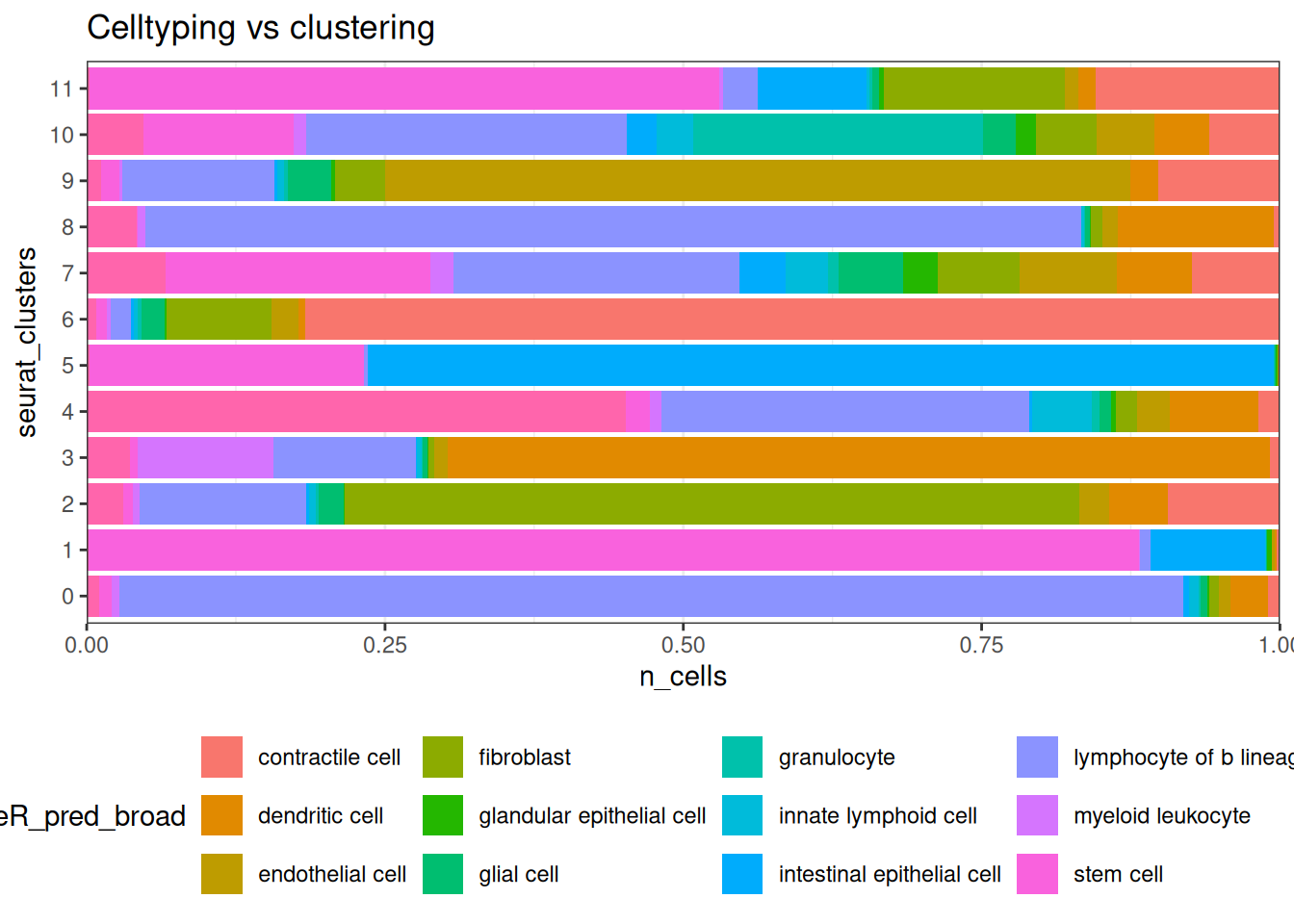
10.5 Spatial examination of plots
The clusters were defined purely on transcriptional similarity, but when plotted on tissue, their location pattern emerges. Here we can see that cluster 1 is epithelial cells.
Plotting both whole sample, and a zoomed in region of just one of the FOVs (in the cosmx definition) within it.
so_sample <- so[, so$tissue_sample=="HC_a"]
ImageDimPlot(so_sample,
             fov          = "GSM7473682.HC.a",
             axes = TRUE,
             border.color = NA, border.size = 0.1,
             cols = 'polychrome', #See DiscretePalette()
             group.by = "seurat_clusters",
             boundaries   = "segmentation",
             crop=TRUE)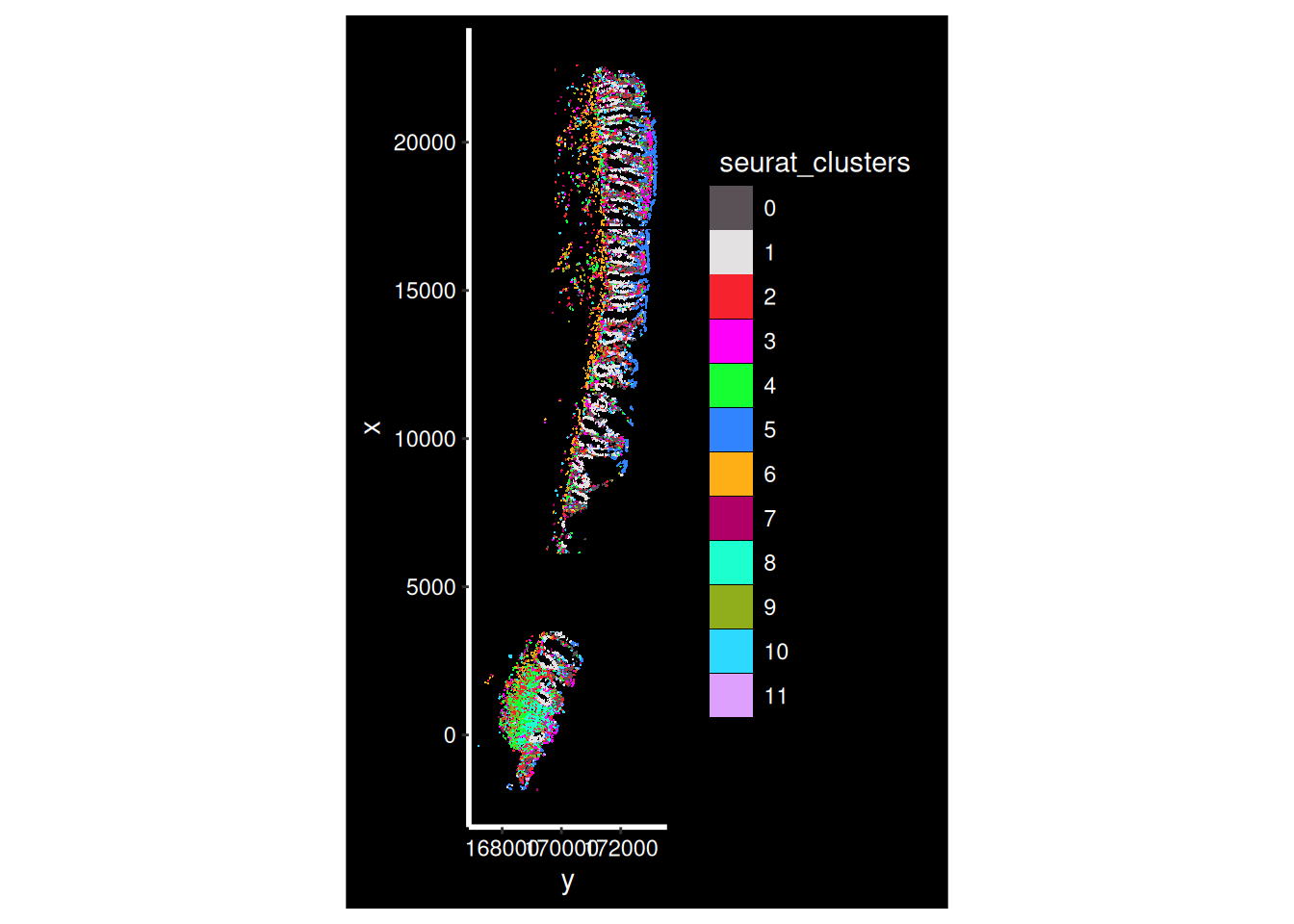
so_fov    <- so_sample[, so_sample$fov==1]
ImageDimPlot(so_fov,
             fov          = "GSM7473682.HC.a",
             axes = TRUE,
             border.color = NA, border.size = 0.1,
             cols = 'polychrome', #See DiscretePalette()
             group.by = "seurat_clusters",
             boundaries   = "segmentation",
             crop=TRUE)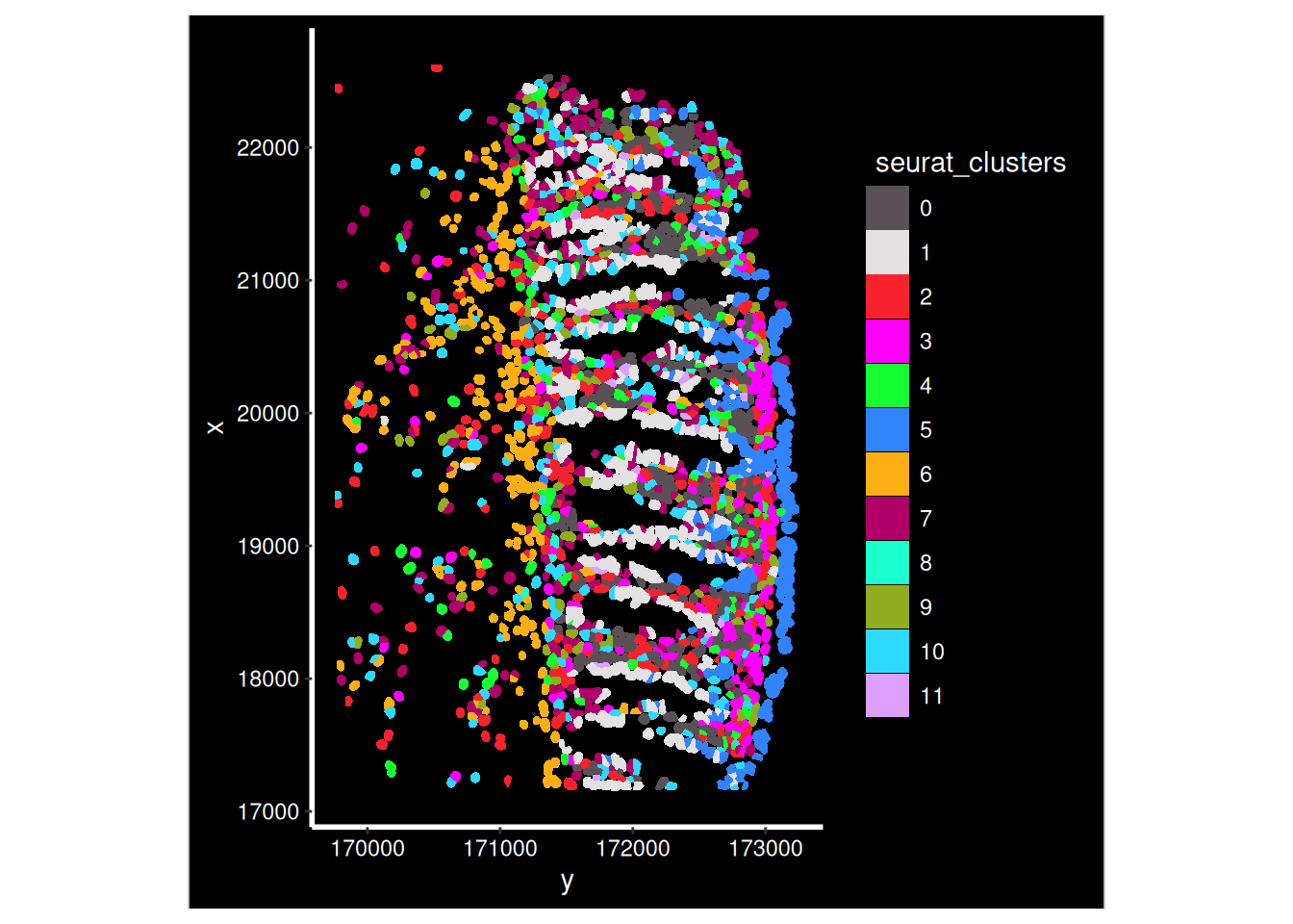
What about the broad predictions?
ImageDimPlot(so_fov,
             fov          = "GSM7473682.HC.a",
             axes = TRUE,
             border.color = NA, border.size = 0.1,
             group.by =  'singleR_pred_broad',
             boundaries   = "segmentation",
             cols = 'polychrome', #See DiscretePalette()
             crop=TRUE)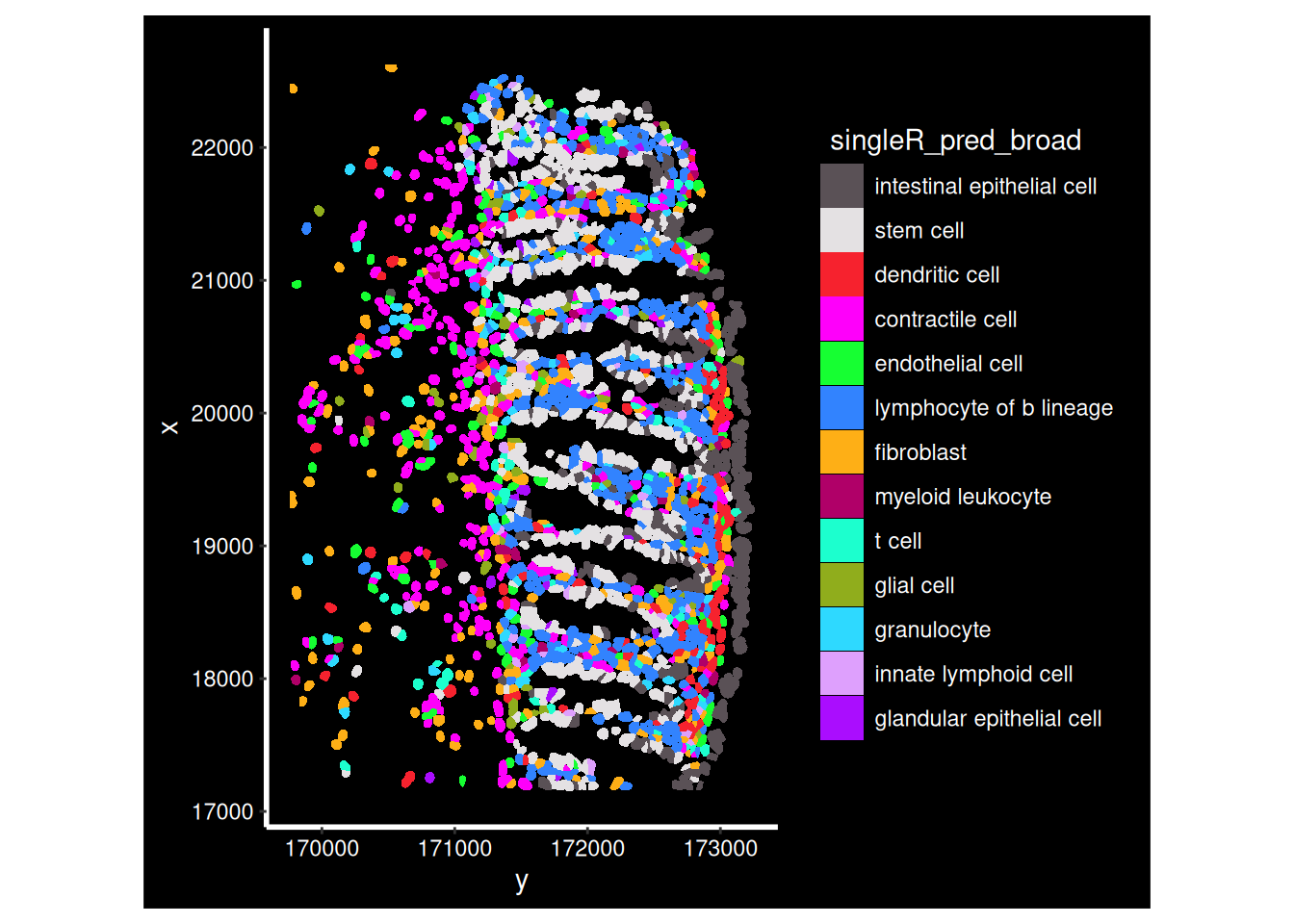
10.6 Using the images data
Image showing colonic mucosa, from https://www.pathologyoutlines.com/topic/colonhistology.html
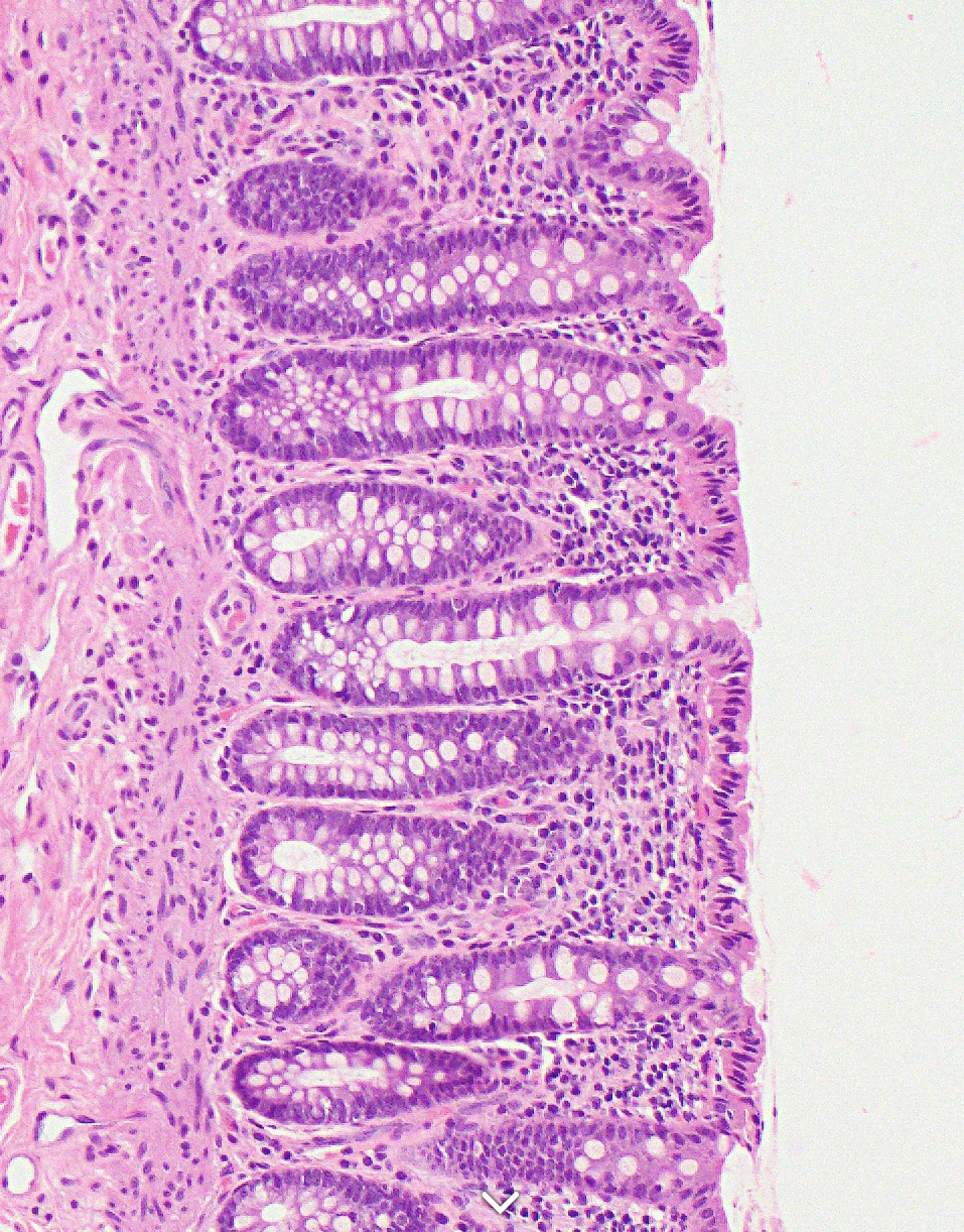
A big advantage of these spatial methods is that you will generally also have H&E or immunofluorescence(IF) (with cell/membrane stains or a full panel) images (and sometimes both), because now you can see the cell.
In imaging data, the ground truth for cell phenotype labels is the morphology of the cell. Even in H&Es, a pathologist can tell the difference between the different white blood cells (lymphocytes, basophils, eosinophils, neutrophils, macrophages etc.). With immunofluoresence, you lose some of this morphology but you gain the additional info of staining patterns - it is a huge advantage to learn how your protein stains are supposed to look and to tell the difference between real signal and noise or non-specific staining. Asking a pathologist who specialises in the tissue you are researching is a huge help when it comes to checking your work!
Of course, the limitations of morphology is that you can’t really tell if it’s a CD4 T cell or CD8 T cell for example, but you should also be able to recognise that if your protein CD4 signal is exclusively in the nucleus, your tissue has problems (fixation? degradation?) and this is not actually a CD4 T cell even if the measured value of CD4 is very high.
Even if we don’t use that directly in the celltype labelling, we can validate our results. We might be fairly confident on some celltypes, however if there’s one that’s giving mixed signals, it can be very helpful to inspect. Sometimes, you notice it’s a mixed cluster, or else two cell populations that are very mixed together and the signals are getting confused. This can help tease the two populations apart. You may find that its clearer to work by by plotting the cell phenotype assignments on the images than on a UMAP.
For an introduction to looking at such images; here are some introductory notes. For protein stains, it can be helpful to compare the staining of your cells to the ones in protein atlas (its not just for RNA!) for the same tissue (although not all of their stains are perfect either). You might also need to align your coordinates with image registration (bioconductor foccused resource).
We won’t cover using image data like this today’s workshop;
- This is an older dataset, and we do not have these images.
- There is currently a lack of support of storing the images in seurat with single cell spatial technologies (it is possible for spot-based visium). But other tools exist e.g. for cosmx, you might pull celltype annotations into napari see guide
10.7 Recording celltype annotations
Note that there are many more tools and approaches for determining celltypes. Especially in the reference based tool space singleR is just one option; See review
It may be worthwhile to seek a method that uses image and positional data in conjunction with transcriptome - it is an active area of research, but for now, singleR was good enough. When seeking such methods, be aware that some methods developed for spot-based technologies (Visium), may not necessarily work or scale to in-situ single cell technologies.
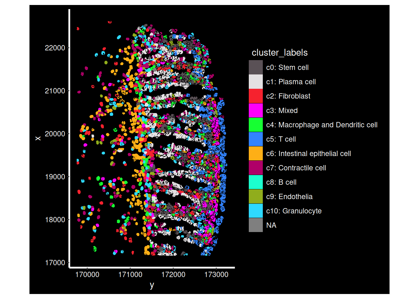
For today, lets apply some celltype labels.
## Apply some cluster names
so$cluster_code <- factor( paste0("c", so$seurat_clusters),   levels=paste0('c', levels(so$seurat_clusters)))
Idents(so) <- so$cluster_code

cluster_content <- list(
  c0 = "Stem cell",
  c1 = "Plasma cell", #B lymphocyte lineage: JCHAIN/ MZB1 / DERL3  (typical for Plasma/Plasma/Plasma)
  c2 = "Fibroblast",
  c3 = "Mixed",
  c4 = "Macrophage and Dendritic cell",  # See detailed predictions, and macrophages are important in this study.
  c5 = "T cell",
  c6 = "Intestinal epithelial cell",  # PIGR
  c7 = "Contractile cell",
  c8 = "B cell",  # B lymphocyte lineage: CD37 / CIITA / IGHM  (B/B/Plasma)
  c9 = "Endothelia",
  c10 = "Granulocyte"
)

# c1 => c1: Stem cell
so$cluster_labels <- factor (
  paste0(names(cluster_content[as.character(so$cluster_code)]), ": ", cluster_content[as.character(so$cluster_code)]) ,
  levels = paste0( names(cluster_content), ": ", cluster_content)
)
so_fov <- so[, so$tissue_sample=="HC_a" & so$fov==1]
ImageDimPlot(so_fov,
             fov          = "GSM7473682.HC.a",
             axes = TRUE,
             border.color = NA, border.size = 0.1,
             cols = 'polychrome',
             group.by = "cluster_labels",
             boundaries   = "segmentation",
             crop=TRUE)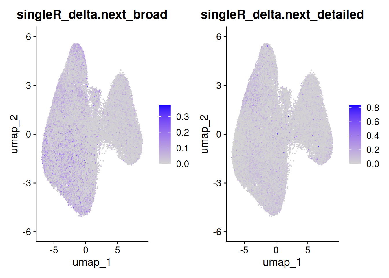
10.8 Pull in real annotation
The authors of this study have shared their actual celltypes. So we can simply directly import their annotation!
annotation_file <- 'data/GSE234713_CosMx_annotation.csv.gz'
anno_table <- read_csv(annotation_file, show_col_types = F)
anno_table <- as.data.frame(anno_table)
rownames(anno_table) <- anno_table$id

so$paper_celltype <- factor(anno_table[colnames(so),]$subset)
so$paper_singleR2 <- factor(anno_table[colnames(so),]$SingleR2)
How many cells per type in the broad set? Where are they on the tissue?
table(so$paper_celltype)##
## epi myeloids plasmas stroma tcells
## 14972 5866 20226 13102 2665
so_fov    <- so[, so$tissue_sample=="HC_a" & so$fov==1]
ImageDimPlot(so_fov,
             fov          = "GSM7473682.HC.a",
             axes = TRUE,
             border.color = NA, border.size = 0.1,
             group.by = "paper_celltype",
             boundaries   = "segmentation",
             crop=TRUE)
The ‘singleR2’ set is very, very detailed! Too much for plotting on the tissue. (NB: They determined their celltypes on their single cell data, which they then used as a reference). The Macrophage subtypes were important in the paper, but we didn’t see a simple macrophage cluster in our clusters. We can do a very quick heatmap to look at how the two classifications compare (this can work better when there are too many celltypes to display nicely with colours). NB: This plot doesn’t view well at small sizes - zoom in to see all the labels.
table(so$paper_singleR2)##
## B cell BEST4 OTOP2
## 1205 1596
## CD4 CD8
## 835 551
## Colonocytes Cycling cells
## 2978 309
## Cycling myeloid Cycling T cells
## 235 57
## Cycling TA DCs
## 332 233
## DN Endothelium
## 140 1943
## Enteroendocrine Eosinophils
## 182 23
## Epithelium Ribhi Fibroblasts
## 952 280
## FRCs GC B cell
## 1390 777
## gd IEL Glia
## 80 734
## Goblet ILC4
## 1915 35
## Inflammatory fibroblasts Inflammatory monocytes
## 1314 102
## M0 M1
## 596 50
## M2 Macrophage NRG1
## 2821 1180
## MAIT Mast
## 265 497
## Memory B cell MT T cells
## 1481 31
## Myofibroblasts N1
## 3689 38
## N2 N3
## 47 44
## Naïve B cell NK
## 2022 40
## Paneth-like PC immediate early response
## 161 1575
## PC IgA PC IgA heat shock
## 316 932
## PC IgA IgM PC IgG
## 3228 8380
## Pericytes Ribhi T cells
## 1259 21
## S1 S2a
## 822 551
## S2b S3
## 658 462
## Secretory progenitor T cells CCL20
## 6445 99
## Tregs Tuft cells
## 511 411
heatmap(table(so$paper_singleR2, so$cluster_labels), Rowv = NA, Colv=NA, margins = c(15, 10)) # base R heatmap - makes margin bigger to fit names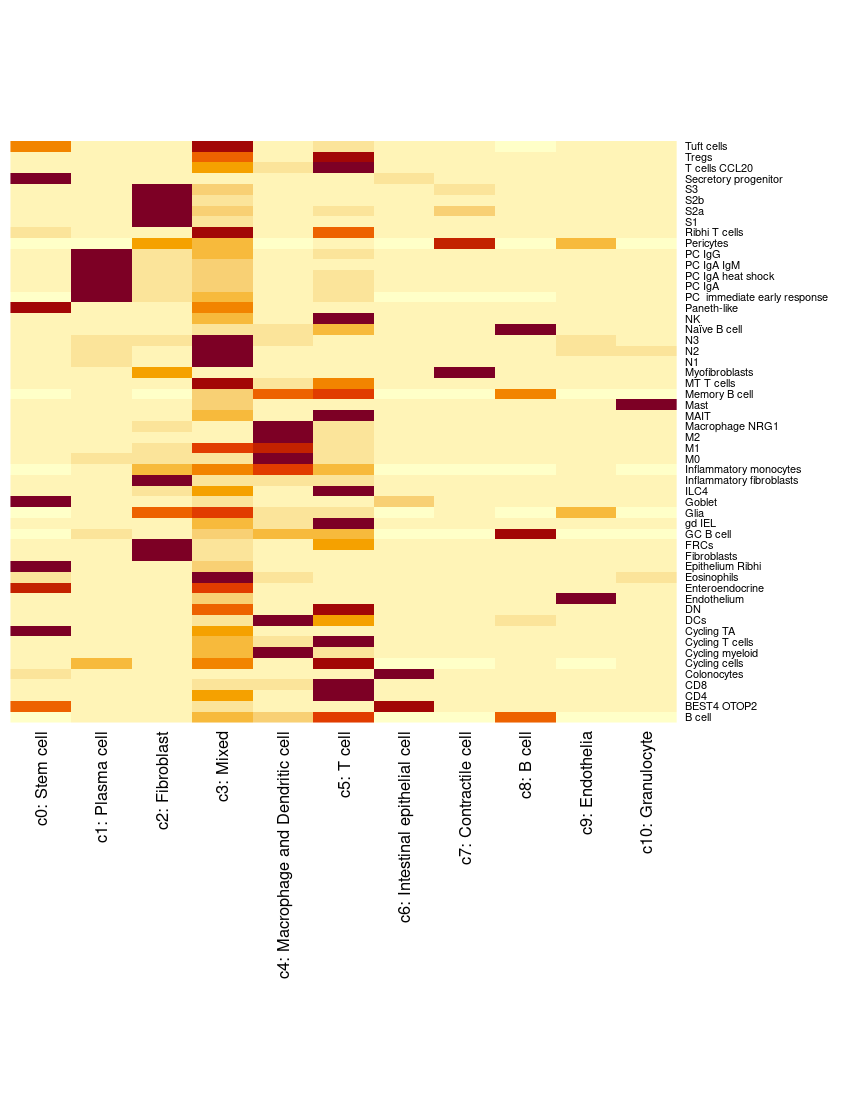
10.9 Save the data
Here would be a natural place to save our annotated data object for downstream analysis;
10.10 Use the annotations!
Now we can do some fun plots with our cell types - for instance to see if there’s change in proportions between samples. You could test this formally with propeller
## Celltype proportions
celltype_summary_table<- so@meta.data %>% as_tibble() %>%
  group_by(condition, tissue_sample, cluster_labels ) %>%
  summarise(n_cells = n())


ggplot(celltype_summary_table, aes(x=tissue_sample, y=n_cells, fill=cluster_labels)) +
  geom_bar(position="fill", stat="identity") +
  theme_bw() +
  coord_flip() +
  theme(legend.position = "bottom") +
  scale_y_continuous(expand = c(0,0)) +
  ggtitle( "Celltype composition") +
  facet_wrap(~condition, ncol = 1, scales = 'free_y')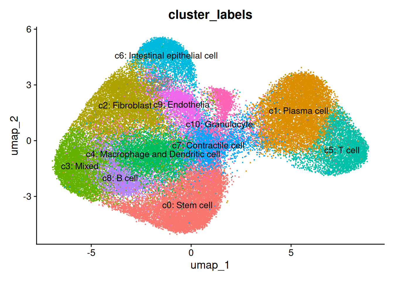
10.11 What about that missing celltype in sample CD_b?
Remember CD_b was missing an area on the UMAP? Corresponding to two clusters? Those were epithelial celltypes, and when we plot it - there’s no epithelia! This data was subsampled from the full dataset.
so_CD_b <- so[, so$tissue_sample=="CD_b"]
ImageDimPlot(so_CD_b,
             fov          = "GSM7473689.CD.b",
             axes = TRUE,
             border.color = NA, border.size = 0.1,
             cols = 'polychrome',
             group.by = "cluster_labels",
             boundaries   = "segmentation",
             crop=TRUE)