Overview

Teaching: 25 min
Exercises: 5 min

Questions

• Use a modern python library and elegant syntax for performance benefits

Objectives

• Intro to Dask concepts and High level datastructures

• Use dask dataframes

• Use dask delayed functions

What is Dask?

Dask is a flexible library for parallel computing in Python.

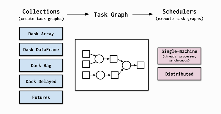
Dask is composed of two parts: Dynamic task scheduling optimized for computation. This is similar to Airflow, Luigi, Celery, or Make, but optimized for interactive computational workloads. “Big Data” collections like parallel arrays, dataframes, and lists that extend common interfaces like NumPy, Pandas, or Python iterators to larger-than-memory or distributed environments. These parallel collections run on top of dynamic task schedulers.

Dask emphasizes the following virtues:

• Familiar: Provides parallelized NumPy array and Pandas DataFrame objects
• Flexible: Provides a task scheduling interface for more custom workloads and integration with other projects.
• Native: Enables distributed computing in pure Python with access to the PyData stack.
• Fast: Operates with low overhead, low latency, and minimal serialization necessary for fast numerical algorithms
• Scales up: Runs resiliently on clusters with 1000s of cores
• Scales down: Trivial to set up and run on a laptop in a single process
• Responsive: Designed with interactive computing in mind, it provides rapid feedback and diagnostics to aid humans

Dask provides high level collections - these are Dask Dataframes, bags, and arrays. On a low level, dask dynamic task schedulers to scale up or down processes, and presents parallel computations by implementing task graphs. It provides an alternative to scaling out tasks instead of threading (IO Bound) and multiprocessing (cpu bound).

Special note regarding dask on Artemis: Dask has a library called dask_jobqueue that allows the pbs specification to be submitted from python script. dask_jobqueue has been known not to work on Artemis due to different interconnects used in head nodes and compute nodes. Please do not use this library and rely on the traditional way we submit jobs to artemis.

Dask Dataframes

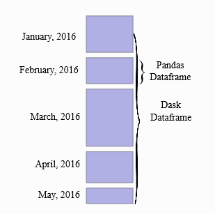
A Dask DataFrame is a large parallel DataFrame composed of many smaller Pandas DataFrames, split along the index. These Pandas DataFrames may live on disk for larger-than-memory computing on a single machine, or on many different machines in a cluster. One Dask DataFrame operation triggers many operations on the constituent Pandas DataFrames.

Common Use Cases: Dask DataFrame is used in situations where Pandas is commonly needed, usually when Pandas fails due to data size or computation speed:

• Manipulating large datasets, even when those datasets don’t fit in memory
• Accelerating long computations by using many cores
• Distributed computing on large datasets with standard Pandas operations like groupby, join, and time series computations

Dask Dataframes may not be the best choice if: your data fits comfortable in RAM - Use pandas only! If you need a proper database. You need functions not implemented by dask dataframes - see Dask Delayed.

Lets begin

If you haven’t done so please activate the conda environment. We will use jupyter notebooks to run python scripts within the /files directory. A major advantage in doing this locally is jupyter notebooks interactive interface, and dask real time diagnostics that provide valuable profiling information.

LOCAL STEPS:

conda activate advpy
jupyter notebook

You should see a jupyter notebook session pop up in your browser.

Locate the /files directory, create a new python 3 file. In this file we will run python scripts to learn dask in an interactive manner.

The below code sets up real time diagnostics provided by dask. Note the shutdown command to perform before quitting this python jupyter notebook session.

from dask.distributed import Client
client = Client()
client
#client.shutdown() to shutdown after done

Diagnostic information on how your efficiently your computational resources are running the code is given when you click the client url. We will cover the basics, but for more info on diagnostics refer to :

Dask Distributed Diagnostics

We will generate some data using one of the python files makedata.py by importing it in ipython.

import makedata
data = makedata.data()
data

The data is preloaded into a dask dataframe. Notice the output to data shows the dataframe metadata.

The concept of splitting the dask dataframe into pandas sub dataframes can be seen by the nopartitians=10 output. This is the number of partitians the dataframe is split into and in this case was automatically calibrated, and can be specified when loading data (npartitians argument). There is a trade off between splitting data too much that improves memory management, and the number of extra tasks it generates.

Let’s inspect the data in its types, and also take the first 5 rows.

By default, dataframe operations are lazy meaning no computation takes place until specified. The .compute() triggers such a computation - and we will see later on that it converts a dask dataframe into a pandas dataframe. head(rows) also triggers a computation - but is really helpful in exploring the underlying data.

data.dtypes
data.head(5)

You should see the below output

In [6]: data.head(5)
Out[6]:
   age     occupation          telephone  ...       street-address          city  income
0   54  Acupuncturist     (528) 747-6949  ...  1242 Gough Crescent  Laguna Beach  116640
1   38   Shelf Filler       111.247.5833  ...       10 Brook Court     Paragould   57760
2   29    Tax Manager       035-458-1895  ...  278 Homestead Trace    Scottsdale   33640
3   19      Publisher  +1-(018)-082-3905  ...     310 Ada Sideline    East Ridge   14440
4   25      Stationer     1-004-960-0770  ...        711 Card Mall     Grayslake   2500

Let’s perform some familiar operations for those who use pandas.

filter operation - filter people who are older than 60 and assign to another dask array called data2

data2 = data[data.age > 60]

Apply a function to a column

data.income.apply(lambda x: x * 1000).head(5)

Assign values to a new column

data = data.assign(dummy = 1)

group by operation - calculate the average incomes by occupation. Notice the compute() trigger that performs the operations.

data.groupby('occupation').income.mean().compute()

A memory efficient style is to create pipelines of operations and trigger a final compute at the end.

datapipe = data[data.age < 20]
datapipe = datapipe.groupby('income').mean()
datapipe.head(4)

        age
income
10240   16.0
11560   17.0
12960   18.0
14440   19.0

Chaining syntax can also be used to do the same thing, but keep readability in your code in mind.

pandasdata = (data[data.age < 20].groupby('income').mean()).compute()

sort operation - get the occupations with the largest people working in them

data.occupation.value_counts().nlargest(5).compute()

write the output of a filter result to csv

data[data.city == 'Madison Heights'].compute().to_csv('Madison.csv')

Custom made operations…. dask.delayed

But what if you need to run your own function, or a function outside of the pandas subset that dask dataframes make available? Dask delayed is your friend. It uses python decorator syntax to convert a function into a lazy executable. The functions can then be applied to build data pipeline operations in a similar manner to what we have just encountered.

A major advantage in turning your functions into delayed (i.e. lazy) functions is that it allows multiple workers to work on contingent functions in an efficient manner. Type in the code below into the python file. The function ‘add’ is contingent on the ‘inc’ and ‘double’ functions. We will make these functions lazy and allow dask to manage resources effiently.

def inc(x):
    return x + 1

def double(x):
    return x * 2

def add(x, y):
    return x + y

data = [1, 2, 3, 4, 5]

output = []
for x in data:
    a = inc(x)
    b = double(x)
    c = add(a, b)
    output.append(c)

total = sum(output)

Dask Delayed Functions Background

On the HPC we can explore a larger example of using dask dataframes and dask delayed functions.

In the /files directory, use your preferred editor to view the complex_system.py file. This script uses dask delayed functions that are applied to a sequence of data using pythonic list comprehension syntax . The code simulates financial defaults in a very theoretical way, and outputs the summation of these predicted defaults.

qsub complex_system.pbs

When that script has completed, the output file testcomplex.o?????? should contain something like this:

Delayed('add-c62bfd969d75abe76f3d8dcf2a9ef99c')
407.5

Exercise 1 - Medium to Difficult:

The above script is a great example of dask delayed functions that are applied to lists, made in an elegant pythonic syntax. Let’s try using these delayed default functions on our data of income and occupations.

Make your own lazy function using the decorator syntax, and perform the computation you have described on a column of the data previously used in the makedata.data() helper file. For bonus points perform an aggregation on this column.

Exercise 2 - Easy:

Given what you know of dask delayed function, please alter the file called computepi_pawsey.py, which calculated estimates of pi without using extra parallel libraries, and alter the code with a dask delayed wrapper to make it lazy and fast

Helpful links

Dask Dataframe intro https://docs.dask.org/en/latest/dataframe.html

API list for Dask Dataframes https://docs.dask.org/en/latest/dataframe.html

What are decorators https://realpython.com/primer-on-python-decorators/

Notes
^1↩As you should recall from the Introduction to Artemis HPC course, the scheduler is the software that runs the cluster, allocating jobs to physical compute resources. Artemis HPC provides us with a separate ‘mini-cluster’ for Training, which has a separate PBS scheduler instance and dedicated resources.

Key Points

• Dask builds on numpy and pandas APIs but operates in a parallel manner

• Computations are by default lazy and must be triggered - this reduces unneccessary computation time