Obesity phase 2 - Comparison of statistical test outcomes on synthetic data when counts vs frequency are different between two groups of publications.

Code

library(here)
library(janitor)
library(readr)
library(dplyr)
library(ggplot2)
library(tidyr)
library(knitr)
library(report)
theme_set(theme_minimal())
library(patchwork)
library(ggfortify)
source(here::here("400_analysis", "functions.R"))

The mean word count of articles in the Australian corpus is:

broadsheet: 810
tabloid: 502

Let’s generate some word counts and then see what happens with data where we have one instance of a particular language type in each article.

Code

broad_wc <- fGarch::rsnorm(1000, mean = 810, sd = 800, xi = 5)
broad_wc <- broad_wc[broad_wc > 0]
tabl_wc <- fGarch::rsnorm(1000, mean = 502, sd = 490, xi = 5)
tabl_wc <- tabl_wc[tabl_wc > 0]

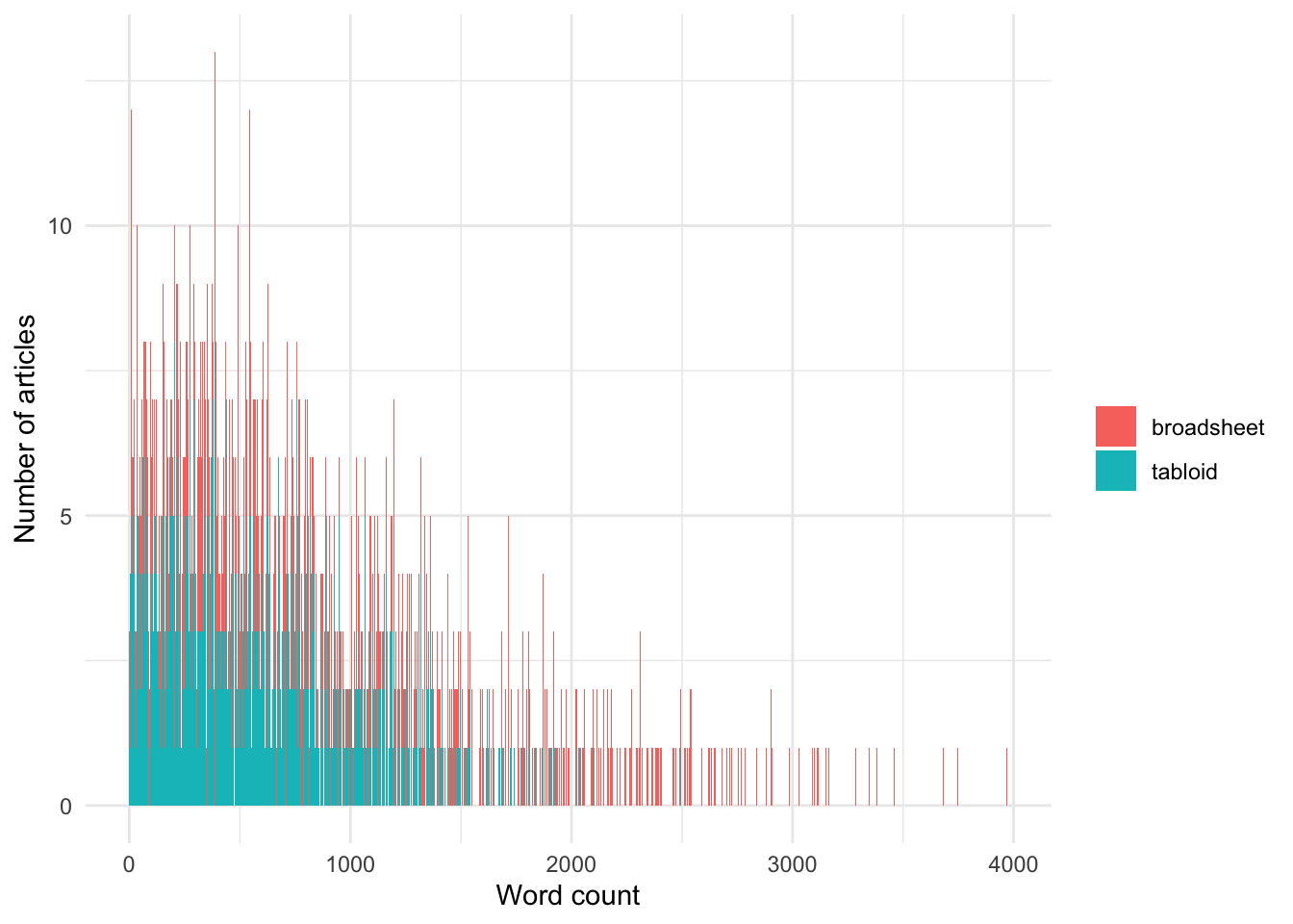
Let’s plot these:

Code

histogram_pairwise(
  wc1 = broad_wc,
  wc2 = tabl_wc,
  label1 = "broadsheet",
  label2 = "tabloid") +
  xlab("Word count") +
  labs(fill = "")

Figure 1: Histogram of the word counts sampled from the distribution for broadsheet and tabloid data.

Now, let’s generate a frequency per thousand words for each of these articles, assuming they each have one instance of the language type (so from a journalist’s perspective, they’ve used the same number of instances in each article).

Code

broad_freq <- 1000/broad_wc
tabl_freq <- 1000/tabl_wc

Note that we observe a SIGNIFICANT difference between the two samples, even though we have simulated them to each feature only ONE instance of the preferred language type.

Code

report::report(t.test(broad_freq, tabl_freq))

The Welch Two Sample t-test testing the difference between broad_freq and tabl_freq (mean of x = 7.88, mean of y = 11.28) suggests that the effect is negative, statistically not significant, and very small (difference = -3.40, 95% CI [-14.19, 7.39], t(1469.60) = -0.62, p = 0.537; Cohen’s d = -0.03, 95% CI [-0.12, 0.06])

Using a non-parametric test does not improve the situation:

Code

mydistribution_custom <- coin::approximate(nresample = 1000,
                              parallel = "multicore",
                              ncpus = 8)
fp_test(
  wc1 = broad_freq,
    wc2 = tabl_freq,
    label1 = "broadsheet",
    label2 = "tabloid",
    dist = mydistribution_custom
)


    Approximative Two-Sample Fisher-Pitman Permutation Test
data:  wc by label (broadsheet, tabloid)
Z = -0.61541, p-value = 0.589
alternative hypothesis: true mu is not equal to 0

Note, however, that using the Chi-square goodness of fit allows us to avoid this issue, when considering the number of articles in each group:

Code

stats::chisq.test(c(length(broad_wc), length(tabl_wc)),
                  p = c(length(broad_wc), length(tabl_wc)),
                  rescale.p = T)


    Chi-squared test for given probabilities
data:  c(length(broad_wc), length(tabl_wc))
X-squared = 0, df = 1, p-value = 1

This does remain an issue when using the Chi-square goodness of fit test when considering the total number of instances:

Code

stats::chisq.test(c(length(broad_wc), length(tabl_wc)),
                  p = c(sum(broad_wc), sum(tabl_wc)),
                  rescale.p = T)


    Chi-squared test for given probabilities
data:  c(length(broad_wc), length(tabl_wc))
X-squared = 102.55, df = 1, p-value < 2.2e-16