Condition-first vs person-first language

In this notebook, we explore whether there is a difference in the use of condition- vs person-first language in the Australian Obesity Corpus.

Executive summary

1. Condition-first language is used in 9-14% of articles from all sources, while person-first language is used in less than 1% of articles.

2. Condition-first language is used in 7-14% of articles per year across the study time period, while person-first language is used in 0.17-1.14% of articles per year.

3. Person-first language is present in approximately the same number of articles in broadsheet and tabloid newspapers, whereas articles with only condition-first language are higher in number in tabloid publications.

• The Pearson’s Chi-squared test with Yates’ continuity correction contrasting articles from tabloids and broadsheets that use only condition-first vs only person-first language indicate a significant link (X-squared = 4.8274, p-value = 0.02801) between type of publication and number of articles using a specific language type. The effect size is quite small (<0.2), indicating that while the result is statistically significant, the fields are weakly associated. So while the number of articles from broadsheet and tabloids that use condition- and person-first language that we observe are different, the magnitude of this difference (i.e. the number of articles we see vs would expect by random chance) is not very high.
• The total number of uses of condition-first language we observe is higher in tabloids and lower in broadsheets than we would expect based on the word count in these subcorpora (p < 0.001).
• The number of articles with condition-first language we observe is also higher in tabloids and lower in broadsheets than we would expect based on the total article count in these subcorpora (p < 0.001).
• The total number of uses of person-first language we observe is somewhat higher in tabloids and lower in broadsheets than we would expect based on the word count in these subcorpora, but this result is not strongly significant (p < 0.05).
• The number of articles with person-first language we observe is, in contrast, lower in tabloids and higher in broadsheets than we would expect based on the total article count in these subcorpora (p < 0.002).

4. Person-first language is present in approximately the same number of articles in left- and right-leaning newspapers, whereas articles with only condition-first language are higher in number in right-leaning publications.

• The total number of uses of condition-first language we observe is higher in right and lower in left-leaning publications than we would expect based on the word count in these subcorpora (p < 0.001).
• The number of articles with condition-first language we observe is also is higher in right and lower in left-leaning publications than we would expect based on the total article count in these subcorpora (p < 0.001).
• The total number of uses of person-first language we observe is higher in left and lower in right-leaning publications than we would expect based on the word count in these subcorpora (p < 0.002).
• The number of articles with person-first language we observe is also is higher in left and lower in right-leaning publications than we would expect based on the total article count in these subcorpora (p < 0.002).
• The Pearson’s Chi-squared test with Yates’ continuity correction contrasting articles from left- and right-leaning publications that use only condition-first vs only person-first language indicate a significant link (X-squared = 4.6405, p-value = 0.03123) between type of publication and number of articles using a specific language type. The effect size is, however, also negligible, indicating that while the result is statistically significant, the fields are weakly associated. This indicates that while we do see more articles that use only condition-first language and fewer that use person-first language in tabloids than in broadsheets, the difference in numbers between these observed number of articles and what we would expect by random chance is not very high.

5. Re-sampling the corpus 10000 times to select 1000 articles at a time without replacement results in a mean of 4 articles per 1000 using person-first language, and 122 per 1000 using condition-first language - so more articles in the corpus use condition-first language than person-first language.

• The Welch Two Sample t-test testing the difference between person_first and condition_first bootstrapping (mean of person_first = 4.11, mean of condition_first = 122.57) suggests that the effect is negative, statistically significant, and large (difference = -118.46, 95% CI [-118.67, -118.26], t(10751.55) = -1138.14, p < .001; Cohen’s d = -16.10, 95% CI [-16.31, -15.88]).

6.In texts that use either condition-first, person-first languages or both, the frequency of condition-first language is higher (mean 4 words per 1000) than person-first (mean 2.7 words per 1000).

• The Welch Two Sample t-test testing the difference between condition_first_frequencies and person_first_frequencies (mean of x = 4.34, mean of y = 2.67) suggests that the effect is positive, statistically significant, and small (difference = 1.66, 95% CI [1.16, 2.17], t(131.59) = 6.49, p < .001; Cohen’s d = 0.44, 95% CI [0.30, 0.58])

7. Relative to the Advertiser, the Age, Australian, Canberra Times, Courier Mail and Sydney Morning Herald had lower frequency of condition-first language.

Code

library(here)
library(dplyr)
library(ggplot2)
library(ggvenn)
library(readr)
library(tidyr)
library(knitr)
library(ggrepel)
library(report)
library(lme4)
library(optimx)
# set ggplot2 to use the minimal theme for all figures in the document
# unless explicitly specified otherwise
theme_set(theme_minimal())
source(here::here("400_analysis", "functions.R"))
condition_first <- read_cqpweb("aoc_all_condition_first.txt")
person_first <- read_cqpweb("aoc_all_person_first.txt")
metadata <- read_csv(here("100_data_raw", "corpus_cqpweb_metadata.csv"))
additional_source_metadata <- read_csv(here("100_data_raw", "addition_source_metadata.csv"))
metadata_full <- inner_join(metadata, additional_source_metadata)
condition_first_annotated <- inner_join(
  metadata_full, condition_first, by = c("article_id" = "text")) %>% 
  mutate(frequency = 10^3*no_hits_in_text/wordcount_total) 
person_first_annotated <- inner_join(
  metadata_full, person_first, by = c("article_id" = "text"))%>% 
  mutate(frequency = 10^3*no_hits_in_text/wordcount_total) 
corpus_articlecounts <- read_csv(here("100_data_raw", "articlecounts_full.csv"), col_names = TRUE, skip = 1) %>% filter(year != "source") %>% rename(source = year)

As discussed in the exploratory data analysis, we use the Python-generated word counts to count the frequency of occurrences per thousand words, as these do not include counts for punctuation symbols and hence do not distort counts for longer texts.

We group articles into tabloids and broadsheets, and by orientation, in the following manner:

Code

metadata_full |>
  select(source, source_type, orientation) |>
  distinct() |>
  kable()

Table 1: Classification of sources into types and by orientation.

source	source_type	orientation
Advertiser	tabloid	right
Australian	broadsheet	right
NorthernT	tabloid	right
CourierMail	tabloid	right
Age	broadsheet	left
SydHerald	broadsheet	left
Telegraph	tabloid	right
WestAus	tabloid	right
CanTimes	broadsheet	left
HeraldSun	tabloid	right
HobMercury	tabloid	right
BrisTimes	broadsheet	left

Total number of articles with each of the language usages

First, we explore how many articles (absolute numbers and relative to the total number of articles in each source) use condition-first vs person-first language.

Code

condition_person_rbound <-
  rbind(
    articles_per_journal(person_first_annotated, "Person-first"),
    articles_per_journal(condition_first_annotated, "Condition-first"))
# generate how many articles per source are in the corpus
corpus_total_articles_bysource <-
  corpus_articlecounts %>% 
  rowwise() %>% 
  mutate(total = sum(c_across(where(is.numeric)))) %>% 
  select(source, total)
condition_person_rbound %>% 
  select(-year) %>% 
  group_by(type) %>% 
  count(source) %>%
  inner_join(corpus_total_articles_bysource) %>%
  mutate(percent = round(100*n/total, 2)) %>%
  rename(count = n) %>%
  pivot_wider(id_cols = source, names_from = type, values_from = c(count, total, percent), names_glue = "{type} {.value}") %>%
  rename(Total_articles = `Person-first total`) %>%
  select(-`Condition-first total`) %>%
  kable()

Table 2: Number and percentage (out of 100%) of articles in which person-first and condition-first language is used in the corpus, by publication.

source	Condition-first count	Person-first count	Total_articles	Condition-first percent	Person-first percent
Advertiser	456	8	3349	13.62	0.24
Age	315	19	2826	11.15	0.67
Australian	191	8	1960	9.74	0.41
BrisTimes	22	1	228	9.65	0.44
CanTimes	212	8	2044	10.37	0.39
CourierMail	434	12	3131	13.86	0.38
HeraldSun	509	14	3722	13.68	0.38
HobMercury	172	2	1465	11.74	0.14
NorthernT	95	2	822	11.56	0.24
SydHerald	430	23	3636	11.83	0.63
Telegraph	144	6	1089	13.22	0.55
WestAus	228	3	1891	12.06	0.16

We can see that condition-first language is used in 9-14% of articles, while person-first language is used in less than 1% of articles across all sources.

Code

corpus_total_articles_byyear <-
  corpus_articlecounts %>%
  pivot_longer(cols = -source, names_to = "year", values_to = "number_of_articles" ) %>%
  select(-source) %>%
  group_by(year) %>%
  summarise(total = sum(number_of_articles)) %>%
  mutate(year = as.numeric(year))
# count the number of articles per source that use person first language
condition_person_rbound %>% 
  select(-source) %>% 
  group_by(type) %>% 
  count(year) %>%
  inner_join(corpus_total_articles_byyear) %>%
  mutate(percent = round(100*n/total, 2)) %>%
  rename(count = n) %>%
  pivot_wider(id_cols = year, names_from = type, values_from = c(count, total, percent), names_glue = "{type} {.value}") %>%
  rename(Total_articles = `Person-first total`) %>%
  select(-`Condition-first total`) %>%
  kable()

Table 3: Number and percentage (out of 100%) of articles in which person-first and condition-first language is used in the corpus, by year.

year	Condition-first count	Person-first count	Total_articles	Condition-first percent	Person-first percent
2008	398	6	3000	13.27	0.20
2009	348	6	2472	14.08	0.24
2010	304	4	2394	12.70	0.17
2011	295	5	2245	13.14	0.22
2012	289	5	2162	13.37	0.23
2013	283	11	2620	10.80	0.42
2014	283	8	2219	12.75	0.36
2015	256	8	2265	11.30	0.35
2016	248	15	1829	13.56	0.82
2017	201	16	1791	11.22	0.89
2018	196	6	1765	11.10	0.34
2019	107	16	1401	7.64	1.14

We can see that condition-first language is used in 7-14% of articles per year across the study time period, while person-first language is used in 0.17-1.14% of articles per year.

Furthermore, the numbers of articles that use person-first language within the corpus are quite small, so we cannot simultaneously explore whether this type of language changes across both publication and year:

Code

assess_year_source(person_first_annotated) 

Table 4: Number of articles that use person-first language by source and year in the Australian Obesity Corpus.

source	2008	2009	2010	2011	2012	2013	2014	2015	2016	2017	2018	2019	Total
Advertiser	1	1	0	0	1	1	0	0	1	2	0	1	8
Age	2	0	1	2	2	1	2	3	2	2	1	1	19
CourierMail	1	0	1	0	0	1	2	1	4	1	1	0	12
HeraldSun	1	0	0	2	0	3	1	0	2	1	1	3	14
SydHerald	1	2	1	1	1	2	1	2	1	3	1	7	23
Australian	0	1	0	0	0	1	0	0	1	2	1	2	8
CanTimes	0	1	0	0	1	2	0	1	0	1	0	2	8
HobMercury	0	1	0	0	0	0	0	0	0	1	0	0	2
WestAus	0	0	1	0	0	0	0	0	1	1	0	0	3
NorthernT	0	0	0	0	0	0	1	1	0	0	0	0	2
Telegraph	0	0	0	0	0	0	1	0	2	2	1	0	6
BrisTimes	0	0	0	0	0	0	0	0	1	0	0	0	1
Total	6	6	4	5	5	11	8	8	15	16	6	16	106

There is also not a lot of articles that use such language from each publication (2-23 articles, mean 9.9 +/- 7.14), so modelling the trend by publication is unlikely to result in meaningful data.

We do have a reasonable number of articles that use condition-first language, so we can model this if desired (except for the Brisbane Times and Daily Telegraph, where we are missing data prior to 2014):

Code

assess_year_source(condition_first_annotated) 

Table 5: Number of articles that use condition-first language by source and year in the Australian Obesity Corpus.

source	2008	2009	2010	2011	2012	2013	2014	2015	2016	2017	2018	2019	Total
Advertiser	40	53	43	49	40	51	43	41	37	25	19	15	456
Age	49	24	24	28	37	25	22	34	26	18	19	9	315
Australian	35	26	20	22	17	11	16	8	9	7	12	8	191
CanTimes	15	18	14	18	24	17	31	24	18	10	19	4	212
CourierMail	65	44	50	31	25	40	38	36	29	29	28	19	434
HeraldSun	66	71	56	61	51	49	35	25	32	28	22	13	509
HobMercury	31	16	15	20	14	23	8	13	8	8	11	5	172
NorthernT	12	21	13	5	7	10	7	5	4	7	3	1	95
SydHerald	47	52	41	35	38	41	30	37	36	23	32	18	430
WestAus	38	23	28	26	36	16	17	14	17	9	3	1	228
BrisTimes	0	0	0	0	0	0	3	5	2	2	5	5	22
Telegraph	0	0	0	0	0	0	33	14	30	35	23	9	144
Total	398	348	304	295	289	283	283	256	248	201	196	107	3208

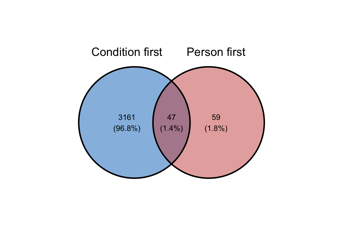
Also, among articles that use person-first language, nearly half will also use condition-first language in the same article:

Code

tmpfig <-
  ggvenn(list(
  `Condition first` = condition_first_annotated$article_id, 
  `Person first` = person_first_annotated$article_id),
  fill_color = c("white", "white"))
ggsave(
  plot=tmpfig,
  device = "png",
       here::here("400_analysis","venn_diagram_condition_person_first.png"),
       bg = "white", 
       width = 4,
       height = 4)
ggvenn(list(
  `Condition first` = condition_first_annotated$article_id, 
  `Person first` = person_first_annotated$article_id),
  fill_color = c("#0073C2FF", "#CD534CFF"))

Figure 1: Number of articles that use person-first, condition-first or both language types within the same article.

This means that comparing the use of person-first and condition-first language using a Chi-square test will not be appropriate, as the same article will be counted towards both condition-first and person-first language.

We can, however, compare the number of articles that use either language type (i.e. ONLY condition-first and only person-first) by type of publication:

Code

language_sourcetype_table <-
  get_article_counts_nooverlap(condition_first_annotated,
                     person_first_annotated,
                     source_type)
language_sourcetype_table %>% 
  kable()

Table 6: Number of articles that use either language type (i.e. ONLY condition-first and only person-first) by type of publication

source_type	condition-first	person-first
broadsheet	1141	30
tabloid	2020	29

We can see that person-first language is present in approximately the same number of articles in broadsheet and tabloid newspapers, whereas articles with only condition-first language are higher in number in tabloid publications.

Code

chisq_source_res <- chisq.test(language_sourcetype_table[,c("condition-first", "person-first")])
prettyrbind_chisq_result(
  df = language_sourcetype_table[,c("condition-first", "person-first")], 
  chisq_source_res, 
  prefix = "corrected") |> kable()

Table 7: Results of Chi-Square test of number of articles that use only person-first and only condition-first language in the corpus.

variable	value
corrected_method	Pearson’s Chi-squared test with Yates’ continuity correction
corrected_parameter	1
corrected_statistic	4.827403
corrected_p.value	0.02801079
corrected_effect_size	0.0387194207367031
corrected_condition_first_observed	1141
corrected_person_first_observed	30
corrected_condition_first_observed	2020
corrected_person_first_observed	29
corrected_condition_first_expected	1149.54378881988
corrected_person_first_expected	21.4562111801242
corrected_condition_first_expected	2011.45621118012
corrected_person_first_expected	37.5437888198758

The Chi-square test results in a p-value that is less than 0.05, indicating a significant link between type of publication and type of language used.

The effect size is quite small (<0.2), indicating that while the result is statistically significant, the fields are only weakly associated.

There has been criticism of use of the Yates correction, so we also provide the uncorrected results below:

Code

chisq_source_res_uncorr <- chisq.test(language_sourcetype_table[,c("condition-first", "person-first")], correct = F)
prettyrbind_chisq_result(
  df = language_sourcetype_table[,c("condition-first", "person-first")], 
  chisq_source_res_uncorr, 
  prefix = "uncorrected") |> kable()

Table 8: Results of Chi-Square test without Yates continuity correction of number of articles that use only person-first and only condition-first language in the corpus.

variable	value
uncorrected_method	Pearson’s Chi-squared test
uncorrected_parameter	1
uncorrected_statistic	5.446196
uncorrected_p.value	0.01961098
uncorrected_effect_size	0.0411262107211088
uncorrected_condition_first_observed	1141
uncorrected_person_first_observed	30
uncorrected_condition_first_observed	2020
uncorrected_person_first_observed	29
uncorrected_condition_first_expected	1149.54378881988
uncorrected_person_first_expected	21.4562111801242
uncorrected_condition_first_expected	2011.45621118012
uncorrected_person_first_expected	37.5437888198758

Let’s next use a similar approach to identify whether left- or right- leaning publications are different in their use of condition- vs person-first language. What is the total number of articles that use EITHER condition-first or person-first language by orientation of publication?

Code

language_orientation_table <- get_article_counts_nooverlap(condition_first_annotated, person_first_annotated, var = orientation)
language_orientation_table %>% kable()

Table 9: Number of articles that use either condition-first or person-first language by orientation of publication.

orientation	condition-first	person-first
left	954	26
right	2207	33

Next, let’s run a Chi-square test on this contingency table:

Code

chisq_language_orientation_corr <- chisq.test(language_orientation_table[,c("condition-first", "person-first")])
prettyrbind_chisq_result(
  df = language_orientation_table[,c("condition-first", "person-first")], 
  chisq_language_orientation_corr, 
  prefix = "corrected") |> kable()

Table 10: Results of Chi-Square test without Yates continuity correction of number of articles that use only person-first and only condition-first language in the corpus.

variable	value
corrected_method	Pearson’s Chi-squared test with Yates’ continuity correction
corrected_parameter	1
corrected_statistic	4.640452
corrected_p.value	0.03122677
corrected_effect_size	0.0379622735273705
corrected_condition_first_observed	954
corrected_person_first_observed	26
corrected_condition_first_observed	2207
corrected_person_first_observed	33
corrected_condition_first_expected	962.04347826087
corrected_person_first_expected	17.9565217391304
corrected_condition_first_expected	2198.95652173913
corrected_person_first_expected	41.0434782608696

The Chi-square test of independence is significant.

However, the effect size is negligible (<= 0.2), indicating that once again the fields are only weakly associated.

There has been criticism of use of the Yates correction, so we also provide the uncorrected results below:

Code

chisq_language_orientation_uncorr <- chisq.test(language_orientation_table[,c("condition-first", "person-first")], correct = F)
prettyrbind_chisq_result(
  df = language_orientation_table[,c("condition-first", "person-first")], 
  chisq_language_orientation_uncorr, 
  prefix = "uncorrected") |> kable()

Table 11: Results of Chi-Square test without Yates continuity correction of number of articles that use only person-first and only condition-first language in the corpus.

variable	value
uncorrected_method	Pearson’s Chi-squared test
uncorrected_parameter	1
uncorrected_statistic	5.276
uncorrected_p.value	0.02162136
uncorrected_effect_size	0.0404785049139109
uncorrected_condition_first_observed	954
uncorrected_person_first_observed	26
uncorrected_condition_first_observed	2207
uncorrected_person_first_observed	33
uncorrected_condition_first_expected	962.04347826087
uncorrected_person_first_expected	17.9565217391304
uncorrected_condition_first_expected	2198.95652173913
uncorrected_person_first_expected	41.0434782608696

Comparing article counts that use condition-first, person-first and no language type

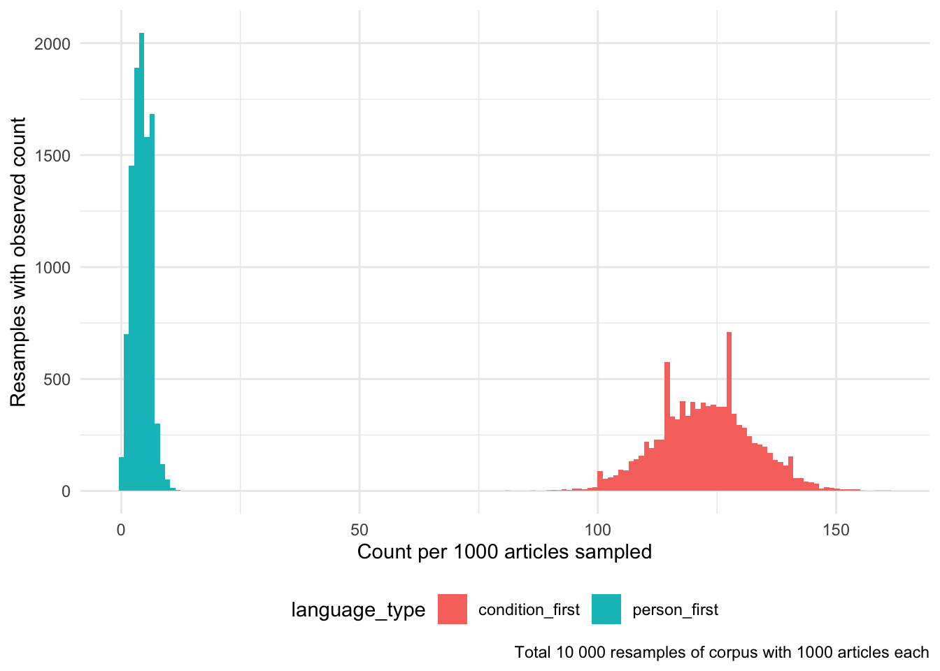
As discussed above, the corpus contains articles that use condition-first, person-first and neither of these two language types. We can use repeated sampling of 1000 articles from the corpus 10000 times to explore how frequently we would observe articles from each of the three groups.

Code

single_row <- function(x) {
  no_hits_cond_first <-
  condition_first_annotated %>% 
  filter(article_id %in% x) %>%
  summarise(count_condition_first = sum(no_hits_in_text)) %>% 
  pull()
no_hits_person_first <-
  person_first_annotated %>% 
  filter(article_id %in% x) %>%
  summarise(count_person_first = sum(no_hits_in_text)) %>% 
  pull()
total_words <-
  metadata_full %>%
  filter(article_id %in% x) %>%
  summarise(wc_total = sum(wordcount_total)) %>% 
  pull()
cbind(data.frame(
  condition_first = sum(x %in% condition_first_annotated$article_id),
  person_first = sum(x %in% person_first_annotated$article_id),
  freq_cond_first = 10^6*no_hits_cond_first/total_words,
  freq_pers_first = 10^6*no_hits_person_first/total_words
))
}
diff_boot <- purrr::map_dfr(
  1:10000,
  ~single_row(sample(metadata_full$article_id, 1000, replace = FALSE))
  )

We can visualise the observed counts per 1000 articles from the 10000 resamples:

Code

diff_boot %>%
  select(-starts_with("freq")) %>%
  pivot_longer(cols = everything(),
               names_to = "language_type", 
               values_to = "count_per_10000_articles") %>%
  ggplot(aes(x = count_per_10000_articles,
             fill = language_type)) +
  geom_histogram(bins = 150) + theme(legend.position = "bottom") + 
  labs(
    x = "Count per 1000 articles sampled",
    y = "Resamples with observed count",
    caption = "Total 10 000 resamples of corpus with 1000 articles each"
  )

Figure 2: Histogram of observed counts of person-first and condition-first language from 10000 resamples of 1000 articles each of the Australian Obesity Corpus.

We can compare the mean of these two observed resamples:

Code

PersonFirst <- diff_boot$person_first
ConditionFirst <- diff_boot$condition_first
report(t.test(PersonFirst, ConditionFirst))

The Welch Two Sample t-test testing the difference between PersonFirst and ConditionFirst (mean of x = 4.03, mean of y = 122.61) suggests that the effect is negative, statistically significant, and large (difference = -118.58, 95% CI [-118.78, -118.38], t(10751.74) = -1151.43, p < .001; Cohen’s d = -16.28, 95% CI [-16.50, -16.06])

This shows that on average of every 1000 articles sampled from the corpus, 4 will use person-first and 122 will use condition-first language.

A non-parametric FP test supports this result:

Code

fp_test(
  wc1 = ConditionFirst,
  wc2 = PersonFirst,
  label1 = "condition",
  label2 = "person", 
  dist = mydistribution
)

    Approximative Two-Sample Fisher-Pitman Permutation Test
data:  wc by label (condition, person)
Z = 140.36, p-value < 1e-04
alternative hypothesis: true mu is not equal to 0

Code

ConditionFirst <- NULL
PersonFirst <- NULL

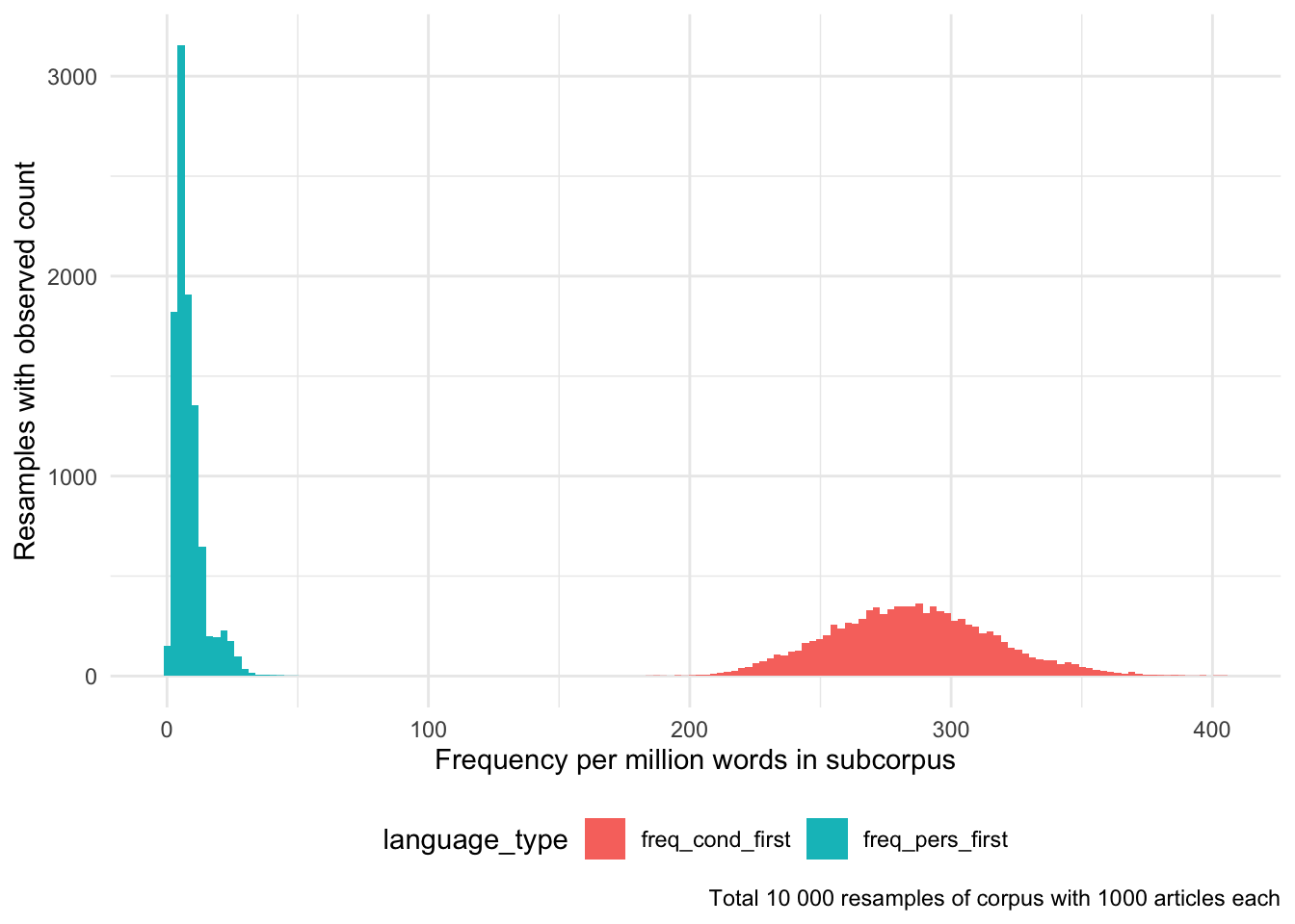
Comparing the frequency of condition-first, person-first and no language type

We can also look at the frequenty of the different language used across the two sets of resamples.

We can visualise the observed frequency per million words from the 10000 resamples:

Code

diff_boot %>%
  select(starts_with("freq")) %>%
  pivot_longer(cols = everything(),
               names_to = "language_type", 
               values_to = "freq_per_million_words") %>%
  ggplot(aes(x = freq_per_million_words,
             fill = language_type)) +
  geom_histogram(bins = 150) + theme(legend.position = "bottom") + 
  labs(
    x = "Frequency per million words in subcorpus",
    y = "Resamples with observed count",
    caption = "Total 10 000 resamples of corpus with 1000 articles each"
  )

Figure 3: Histogram of frequency per million words in subcorpus of person-first and condition-first language from 10000 resamples of 1000 articles each of the Australian Obesity Corpus.

We can compare the mean of these two observed resamples:

Code

ConditionFirst <- diff_boot$freq_cond_first
PersonFirst <- diff_boot$freq_pers_first
report(t.test(PersonFirst, 
              ConditionFirst))

The Welch Two Sample t-test testing the difference between PersonFirst and ConditionFirst (mean of x = 8.23, mean of y = 284.87) suggests that the effect is negative, statistically significant, and large (difference = -276.64, 95% CI [-277.26, -276.01], t(10658.76) = -870.06, p < .001; Cohen’s d = -12.30, 95% CI [-12.47, -12.14])

This shows that on average of every 1000 articles sampled from the corpus, 4 will use person-first and 122 will use condition-first language.

A non-parametric FP test confirms this result:

Code

fp_test(
  wc1 = ConditionFirst,
  wc2 = PersonFirst,
  label1 = "condition",
  label2 = "person", 
  dist = mydistribution
)

    Approximative Two-Sample Fisher-Pitman Permutation Test
data:  wc by label (condition, person)
Z = 139.59, p-value < 1e-04
alternative hypothesis: true mu is not equal to 0

Comparing the number of phrases that use condition-first vs person-first language

We can also take a different approach, comparing the number of phrases that use each language type; Here each phrase will contribute only to one group, i.e. be counted towards either person-first or condition-first. A phrase is defined in this context as an instance of language use, for example the article “AD150801123” contains 7 phrases, numbered below, that are classified by CQPweb as condition-first language:

The discovery by the Murdoch Childrens Institute raises hope that if we can tackle obesity in childhood(1) we can avoid a tsunami of obesity-related(2) health expenses in the future.

<..> “The findings will have major implications for how we treat childhood obesity(3),” says Professor Sabin.

A review by the Murdoch Childrens Research Institute published in the Journal of Paediatrics and Child Health has found childhood obesity(4) has doubled in prevalence since the 1980s. Professor Sabin says while rates of childhood overweight and obesity(5) have plateaued the severity of the problem has increased.

“Childhood obesity(6) has become a global crisis and is one of the world’s most pressing public health issues,” he says.The Murdoch Childrens Institute is undertaking a number of studies and programs to combat childhood obesity(7).

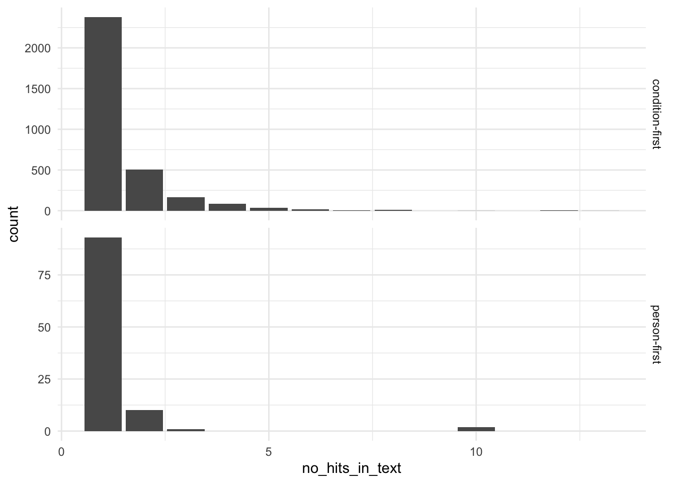
We do, however, need to confirm that most articles have a small number of phrases, vs a small number of articles with a large number of phrases fully underpinning our counts. Let’s look at how many articles have how many counts of each language usage:

Code

count_language_types <- condition_first_annotated %>%
  dplyr::select(article_id, no_hits_in_text) %>%
  mutate(type="condition-first") %>%
  rbind({
    person_first_annotated %>%
      select(article_id, no_hits_in_text) %>%
      mutate(type="person-first")
  })
count_language_types %>% 
  group_by(no_hits_in_text, type) %>%
  count() %>%
  pivot_wider(names_from=type, values_from = n, values_fill = 0) %>%
  kable()

Table 12: CQP-web determined number of hits in text, of condition-first and person-first language.

no_hits_in_text	condition-first	person-first
1	2379	93
2	508	10
3	165	1
4	82	0
5	35	0
6	19	0
7	5	0
8	11	0
10	1	2
12	2	0
13	1	0

Code

count_language_types %>%
  ggplot(aes(x = no_hits_in_text)) + geom_bar() + facet_grid(type~., scales = "free_y")

Figure 4: Histogram of CQP-web determined number of hits in text, of condition-first and person-first language.

Most articles have 1-2 uses of person-first/condition-first language, but some have up to 13 uses. How many total instances are there?

Code

count_language_types %>% 
  group_by(type) %>% 
  summarise( instances = sum(no_hits_in_text),
             articles = n()) %>%
  kable()

Table 13: Total number of CQP-web determined instances and articles with at least one instance of condition-first and person-first language.

type	instances	articles
condition-first	4677	3208
person-first	136	106

Relative frequency of condition- vs person-first language

Let’s explore what the relative frequency, calculated as 10^3*no_hits_in_text/wordcount_total (where no_hits_in_text is determined by CQPweb and wordcount_total is the Python word count), of condition-first vs person-first language looks like.

Code

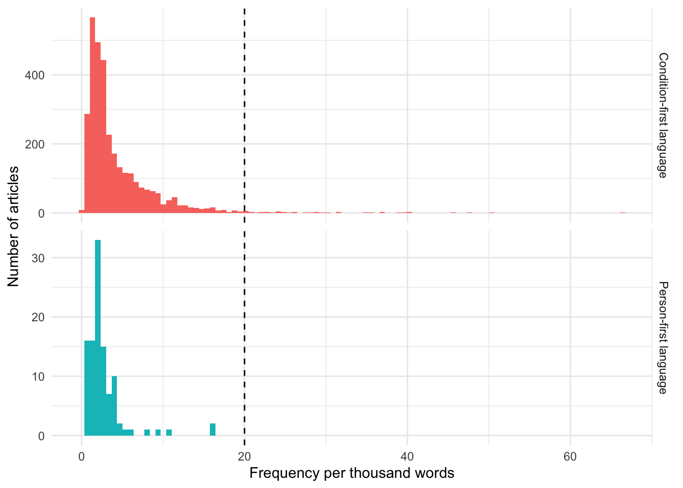
freq_1 <- condition_first_annotated %>%
  select(frequency) %>%
  mutate(condition = "Condition-first language") %>%
  rbind({
  person_first_annotated %>%
  select(frequency) %>%
  mutate(condition = "Person-first language")
  }) 
freq_1_gt100words <- condition_first_annotated %>%
  filter(wordcount_from_metatata >= 100) %>%
  select(frequency) %>%
  mutate(condition = "Condition-first language") %>%
  rbind({
  person_first_annotated %>%
  filter(wordcount_from_metatata >= 100) %>%
  select(frequency) %>%
  mutate(condition = "Person-first language")
  }) 
freq_1 %>%
  ggplot(aes(x = frequency, fill = condition)) +
  facet_grid(condition~., scales = "free_y") +
  geom_histogram(bins = 100) + 
  xlab("Frequency per thousand words") + 
  ylab("Number of articles") + theme(legend.position = "none") +
  geom_vline(xintercept = 20, lty=2)

Figure 5: Histogram of relative frequency per 1000 words of condition-first and person-first language in the Australian Obesity Corpus.

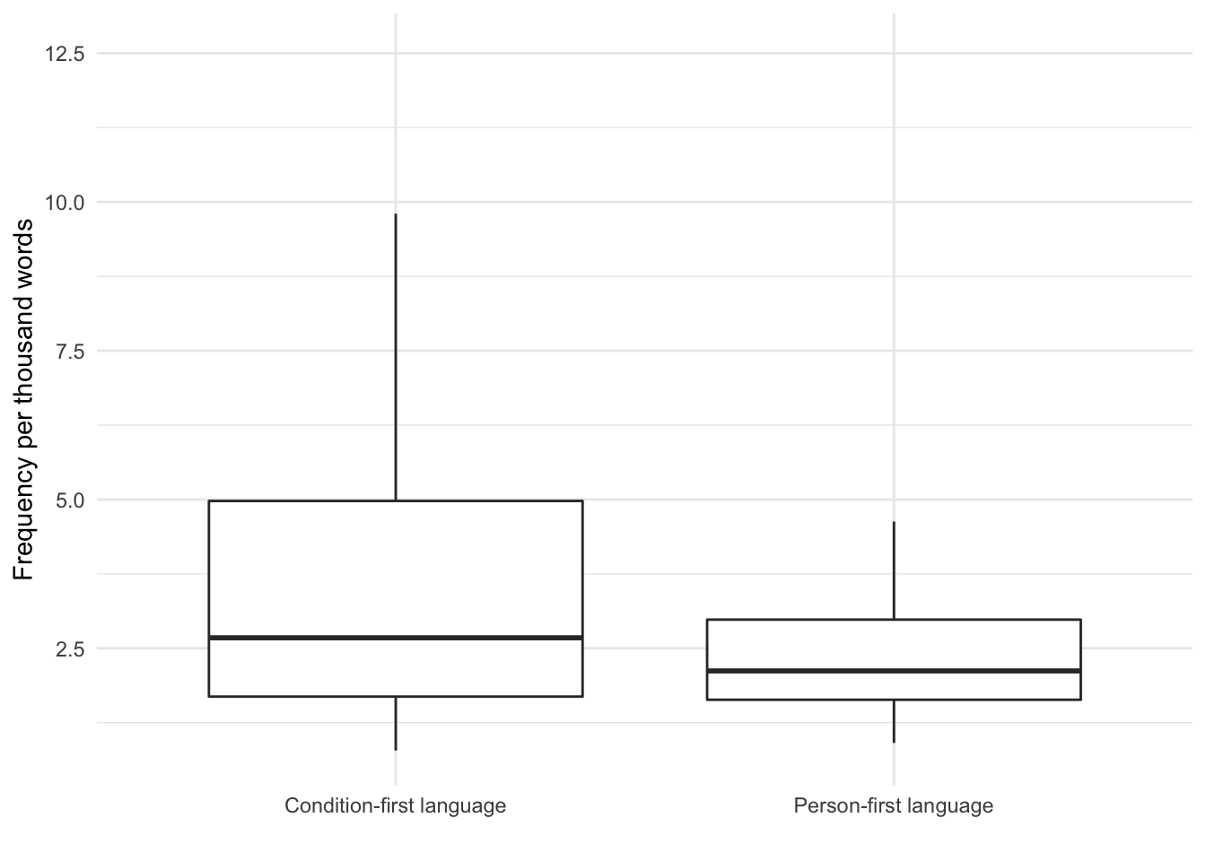
Let’s create a box plot to compare the frequency per thousand words:

Code

freq_1 %>%
  ggplot(aes( y =  frequency, x = condition)) + 
  geom_boxplot(outlier.shape = NA) +
  scale_y_continuous(limits = quantile(freq_1$frequency, c(0.05, 0.95))) +
  labs(
    x = "",
    y = "Frequency per thousand words"
  )

Figure 6: Box plot comparing the distribution of the relative frequency per 1000 words of condition-first and person-first language in the Australian Obesity Corpus.

We can then use a two-sample t-test to compare the mean frequency of condition-first vs person-first language in the corpus:

Code

condition_first_frequencies <- freq_1 %>% 
  filter(condition == "Condition-first language") %>% 
  pull(frequency)
person_first_frequencies <- freq_1 %>%
  filter(condition == "Person-first language") %>% 
  pull(frequency)
report(t.test(condition_first_frequencies,
       person_first_frequencies
       ))

The Welch Two Sample t-test testing the difference between condition_first_frequencies and person_first_frequencies (mean of x = 4.34, mean of y = 2.67) suggests that the effect is positive, statistically significant, and small (difference = 1.66, 95% CI [1.16, 2.17], t(131.59) = 6.49, p < .001; Cohen’s d = 0.44, 95% CI [0.30, 0.58])

In texts that use either condition-first, person-first languages or both, the frequency of condition-first language is higher (mean 4 words per 1000) than person-first (mean 2.7 words per 1000).

We can also use a non-parametric FP test to support this:

Code

fp_test(
  wc1 = condition_first_frequencies,
  wc2 = person_first_frequencies,
  label1 = "condition",
  label2 = "person", 
  dist = mydistribution
)

    Approximative Two-Sample Fisher-Pitman Permutation Test
data:  wc by label (condition, person)
Z = 3.5855, p-value = 0.0012
alternative hypothesis: true mu is not equal to 0

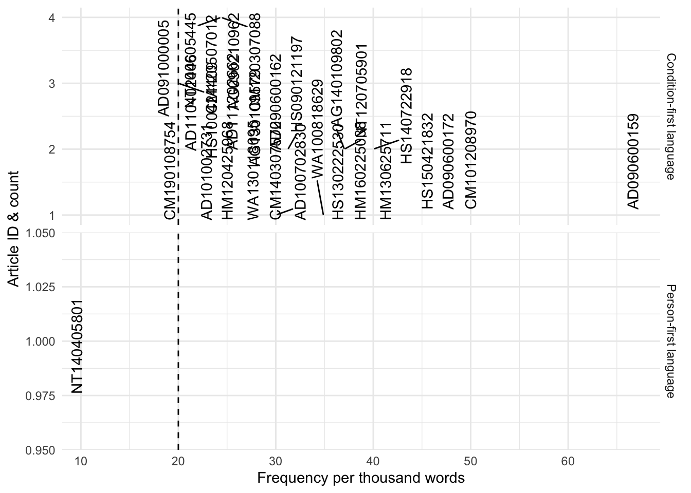
The below plot shows the article ids of articles with a word count less than 100 for person-first language, and article ids with word counts less than 100 where the frequency is greater than 20 for condition-first language

Code

condition_first_annotated %>%
  # select only texts less than 100 words
  filter(wordcount_total <= 100) %>%
  select(article_id, frequency) %>%
  mutate(condition = "Condition-first language") %>%
  # note that for condition-first only looking at those that are very high frequency here
  filter(frequency >= 20) %>%
  rbind({
  person_first_annotated %>%
  # select only texts less than 100 words
  filter(wordcount_total <= 100) %>%
  select(article_id, frequency) %>%
  mutate(condition = "Person-first language")
  }) %>% 
  group_by(frequency) %>%
  mutate(cnt = n()) %>%
  ggplot(aes(x = frequency, y = cnt, fill = condition, label = article_id)) +
  facet_grid(condition~., scales = "free_y") +
  geom_text_repel(check_overlap = TRUE, angle = 90) +
  xlab("Frequency per thousand words") + 
  ylab("Article ID & count") + theme(legend.position = "none") +
  geom_vline(xintercept = 20, lty=2)

Figure 7: Article ids of articles with (top) word counts less than 100 where the frequency is greater than 20 for condition-first language, and (bottom) a word count less than 100 for person-first language.

There are a few texts with very high frequencies. These mostly occur in cases where the text length itself is quite short. We can consider whether we want to filter out texts with a word count of less than 100 words.

If we run a t-test on the dataset filtered to only contain texts greater than 100 words, we can see that while the results are still significant, the mean difference is less.

Code

condition_first_frequencies_gt100 <- freq_1_gt100words %>% 
  filter(condition == "Condition-first language") %>% 
  pull(frequency)
person_first_frequencies_gt100 <- freq_1_gt100words %>%
  filter(condition == "Person-first language") %>% 
  pull(frequency)
report(t.test(
  condition_first_frequencies_gt100,
  person_first_frequencies_gt100
       ))

The Welch Two Sample t-test testing the difference between condition_first_frequencies_gt100 and person_first_frequencies_gt100 (mean of x = 3.69, mean of y = 2.60) suggests that the effect is positive, statistically significant, and small (difference = 1.10, 95% CI [0.62, 1.57], t(118.21) = 4.58, p < .001; Cohen’s d = 0.38, 95% CI [0.21, 0.55])

This is supported by a non-parametric FP test:

Code

fp_test(
  wc1 = condition_first_frequencies_gt100,
  wc2 = person_first_frequencies_gt100,
  label1 = "condition",
  label2 = "person", 
  dist = mydistribution
)

    Approximative Two-Sample Fisher-Pitman Permutation Test
data:  wc by label (condition, person)
Z = 3.3794, p-value = 8e-04
alternative hypothesis: true mu is not equal to 0

Person-first language frequency

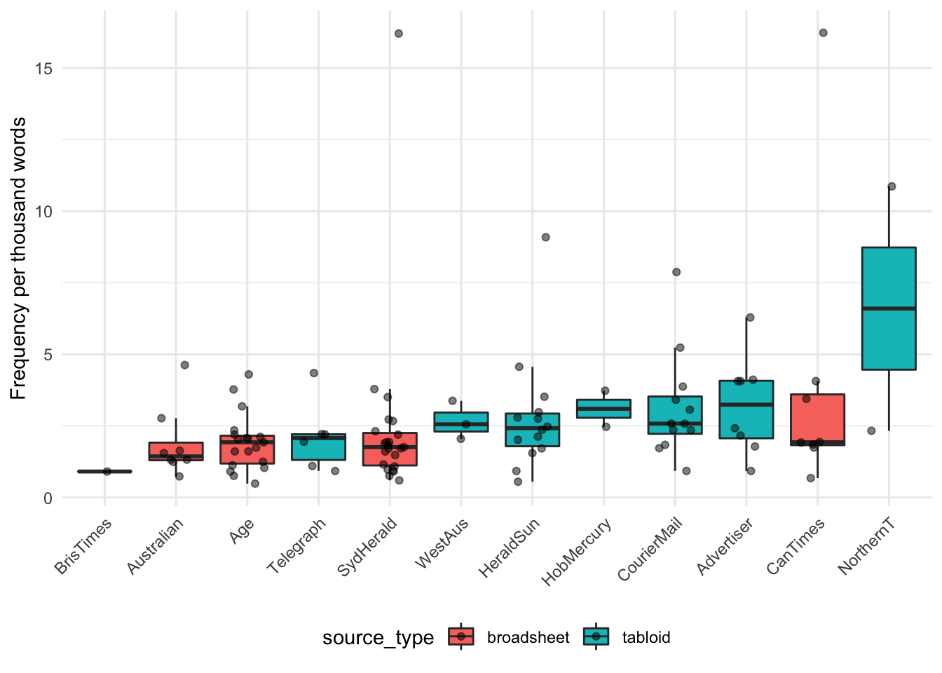
Let’s visualise the frequency, calculated as 10^3*no_hits_in_text/wordcount_total (where no_hits_in_text is determined by CQPweb and wordcount_total is the Python word count), of person-first language by publication:

Code

person_first_annotated %>%
  select(source, frequency, year, source_type) %>%
  ggplot(aes(x = reorder(source, frequency), 
             y = frequency, 
             fill = source_type)) +
  geom_boxplot(outlier.shape = NA) + 
  theme(axis.text.x=element_text(angle = 45, hjust =1),
        legend.position = "bottom") +
  labs(x = NULL, 
       y = "Frequency per thousand words") +
  geom_jitter(width = 0.25, alpha = 0.5) 

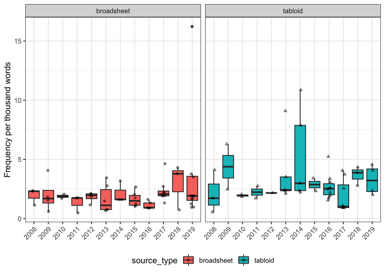
Figure 8: Box and jitter plot showing the summary statistics and raw values of the frequency per 1000 words of person-first language in the different sources, with boxes coloured based on source type. This shows, for example, that the Northern Territorian has the highest median frequncy of person-first language, but this is because the summary statistics are only based on two quite divergent data points.

And per year:

Code

person_first_annotated %>%
  select(source, frequency, year, source_type) %>%
  ggplot(aes(x = as.factor(year), y = frequency, 
             fill = source_type,  shape = source_type)) +
  facet_wrap(~source_type) +
  geom_boxplot(outlier.shape = NA) + theme_bw() +
  theme(axis.text.x=element_text(angle = 45, hjust =1),
        legend.position = "bottom") +
  labs(x = NULL, y = "Frequency per thousand words") +
  geom_jitter(width = 0.1, alpha = 0.5) 

Figure 9: Box and jitter plot showing the summary statistics and raw values of the frequency per 1000 words of person-first language by year and source type. This shows that due to the low numbers of articles using person-first language, there is substantial variability in the summary statistics (median, IQR) across the years.

Condition- and person-first language normalised by total article length

We can also look at the frequency of person-first and condition-first language by dividing the number of observations of each language type by the total word count of articles in which they are found (i.e. frequency per 1000 words not on a per-article basis, but on a per total word count of articles in the group).

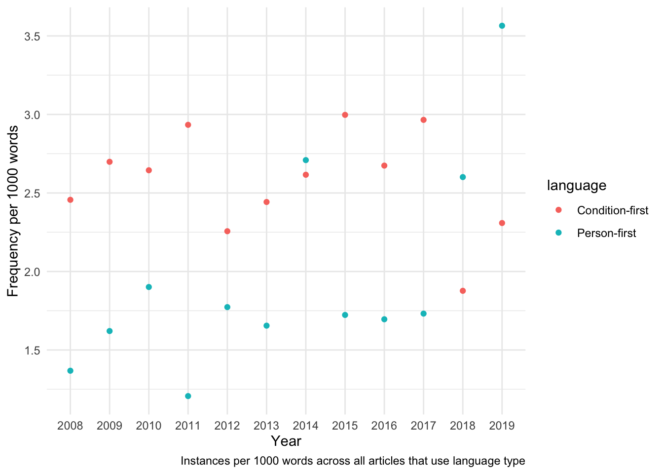
For example, in the table below, there are 6 instances of person-first language in 2008, and the total word count of the articles that contain these 6 instances is 4386 words. Therefor, the normalised frequency is 6*1000/4386 = 1.37.

Code

freq_per_subcorpus <- function(df, group_vars){
  df %>%
  group_by(!!!group_vars) %>%
  summarise(
    total_instances = sum(no_hits_in_text),
    total_wc = sum(wordcount_total),
    instances_per_1000 = 1000 * total_instances/total_wc
  )
}
inner_join(
  {freq_per_subcorpus(person_first_annotated, 
                      group_vars=vars(year)) %>%
      rename("instances_person_first" = "total_instances",
             "wc_personfirst" = "total_wc",
             "person first instances per 1000 words" = "instances_per_1000")
  },
  {freq_per_subcorpus(
    condition_first_annotated, 
    group_vars=vars(year)) %>%
      rename("instances_cond_first" = "total_instances",
             "wc_condfirst" = "total_wc",
             "condition first instances per 1000 words" = "instances_per_1000")
  }) %>% kable(digits = 2)

Table 14: Number of instances of the two language types by year, total word count of articles that use the specified language type and the relative frequency of instances per 1000 words across all articles that year.

year	instances_person_first	wc_personfirst	person first instances per 1000 words	instances_cond_first	wc_condfirst	condition first instances per 1000 words
2008	6	4386	1.37	553	225124	2.46
2009	7	4319	1.62	507	187891	2.70
2010	4	2104	1.90	452	170920	2.64
2011	5	4144	1.21	447	152357	2.93
2012	5	2820	1.77	385	170630	2.26
2013	12	7251	1.65	382	156399	2.44
2014	9	3322	2.71	408	155966	2.62
2015	9	5223	1.72	436	145468	3.00
2016	15	8846	1.70	388	145091	2.67
2017	18	10394	1.73	309	104202	2.97
2018	9	3460	2.60	273	145452	1.88
2019	37	10379	3.56	137	59344	2.31

Code

rbind({freq_per_subcorpus(person_first_annotated, 
                   group_vars=vars(year)) %>%
    mutate(language = "Person-first")},
      {freq_per_subcorpus(condition_first_annotated, 
                   group_vars=vars(year)) %>%
    mutate(language = "Condition-first")}
        ) %>%
  ggplot(aes(x = as.factor(year),
             y = instances_per_1000,
             col = language)) +
  geom_point() +
  labs(x = "Year",
       y = "Frequency per 1000 words",
       caption = "Instances per 1000 words across all articles that use language type")

Figure 10: Visualisation of the above relative frequency per 1000 words of person-first and condition-first language by year.

We can also look at this across sources:

Code

inner_join(
  {freq_per_subcorpus(person_first_annotated, 
                      group_vars=vars(source)) %>%
      rename("instances_person_first" = "total_instances",
             "wc_personfirst" = "total_wc",
             "person first instances per 1000 words" = "instances_per_1000")
  },
  {freq_per_subcorpus(
    condition_first_annotated, 
    group_vars=vars(source)) %>%
      rename("instances_cond_first" = "total_instances",
             "wc_condfirst" = "total_wc",
             "condition first instances per 1000 words" = "instances_per_1000")
  }) %>% kable(digits = 2)

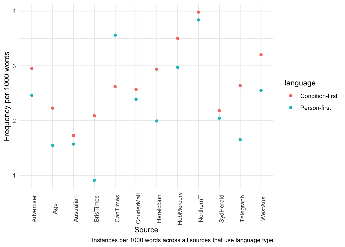
Table 15: Number of instances of the two language types by source, total word count of articles that use the specified language type and the relative frequency of instances per 1000 words across all articles from that source.

source	instances_person_first	wc_personfirst	person first instances per 1000 words	instances_cond_first	wc_condfirst	condition first instances per 1000 words
Advertiser	9	3655	2.46	636	215470	2.95
Age	21	13586	1.55	509	228541	2.23
Australian	10	6368	1.57	283	163862	1.73
BrisTimes	1	1101	0.91	35	16760	2.09
CanTimes	17	4774	3.56	342	130561	2.62
CourierMail	12	5018	2.39	607	236038	2.57
HeraldSun	16	8030	1.99	705	239849	2.94
HobMercury	2	673	2.97	240	68552	3.50
NorthernT	2	521	3.84	120	30149	3.98
SydHerald	37	18111	2.04	697	319498	2.18
Telegraph	6	3636	1.65	186	70524	2.64
WestAus	3	1175	2.55	317	99040	3.20

Code

rbind({freq_per_subcorpus(person_first_annotated, 
                   group_vars=vars(source)) %>%
    mutate(language = "Person-first")},
      {freq_per_subcorpus(condition_first_annotated, 
                   group_vars=vars(source)) %>%
    mutate(language = "Condition-first")}
        ) %>%
  ggplot(aes(x = source,
             y = instances_per_1000,
             col = language)) +
  geom_point() +
  labs(x = "Source",
       y = "Frequency per 1000 words",
       caption = "Instances per 1000 words across all sources that use language type") +
  theme(axis.text.x = element_text(angle=90))

Figure 11: Visualisation of the above relative frequency per 1000 words of person-first and condition-first language by source.

We can also do this across source and year:

Code

inner_join(
  {freq_per_subcorpus(person_first_annotated, 
                      group_vars=vars(source, year)) %>%
      rename("instances_person_first" = "total_instances",
             "wc_personfirst" = "total_wc",
             "person first instances per 1000 words" = "instances_per_1000")
  },
  {freq_per_subcorpus(
    condition_first_annotated, 
    group_vars=vars(source, year)) %>%
      rename("instances_cond_first" = "total_instances",
             "wc_condfirst" = "total_wc",
             "condition first instances per 1000 words" = "instances_per_1000")
  }) %>% kable(digits = 2)

Table 16: Number of instances of the two language types by source, year, total word count of articles that use the specified language type and the relative frequency of instances per 1000 words across all articles from that source that year.

source	year	instances_person_first	wc_personfirst	person first instances per 1000 words	instances_cond_first	wc_condfirst	condition first instances per 1000 words
Advertiser	2008	1	243	4.12	49	13109	3.74
Advertiser	2009	1	159	6.29	69	22082	3.12
Advertiser	2012	1	462	2.16	58	20250	2.86
Advertiser	2013	1	413	2.42	67	22586	2.97
Advertiser	2016	1	561	1.78	52	19254	2.70
Advertiser	2017	3	1571	1.91	40	12681	3.15
Advertiser	2019	1	246	4.07	21	7529	2.79
Age	2008	2	1316	1.52	68	36713	1.85
Age	2010	1	487	2.05	44	13081	3.36
Age	2011	2	2630	0.76	47	13058	3.60
Age	2012	2	953	2.10	49	27123	1.81
Age	2013	1	1319	0.76	34	21790	1.56
Age	2014	2	935	2.14	33	14387	2.29
Age	2015	3	2257	1.33	79	25206	3.13
Age	2016	2	1721	1.16	48	20528	2.34
Age	2017	2	973	2.06	26	14002	1.86
Age	2018	2	465	4.30	31	20118	1.54
Age	2019	2	530	3.77	10	6019	1.66
Australian	2009	2	1289	1.55	50	22444	2.23
Australian	2013	1	361	2.77	13	7129	1.82
Australian	2016	1	758	1.32	15	9868	1.52
Australian	2017	3	1188	2.53	9	5008	1.80
Australian	2018	1	1357	0.74	14	11260	1.24
Australian	2019	2	1415	1.41	11	6369	1.73
BrisTimes	2016	1	1101	0.91	3	1661	1.81
CanTimes	2009	1	246	4.07	23	8318	2.77
CanTimes	2012	1	539	1.86	32	14363	2.23
CanTimes	2013	2	1764	1.13	29	10193	2.85
CanTimes	2015	1	573	1.75	48	12869	3.73
CanTimes	2017	1	520	1.92	21	6585	3.19
CanTimes	2019	11	1132	9.72	8	2428	3.29
CourierMail	2008	1	580	1.72	92	44008	2.09
CourierMail	2010	1	543	1.84	72	29876	2.41
CourierMail	2013	1	425	2.35	60	24932	2.41
CourierMail	2014	2	550	3.64	51	13082	3.90
CourierMail	2015	1	293	3.41	50	15976	3.13
CourierMail	2016	4	1292	3.10	41	10375	3.95
CourierMail	2017	1	1077	0.93	44	11410	3.86
CourierMail	2018	1	258	3.88	38	18314	2.07
HeraldSun	2008	1	1815	0.55	90	31663	2.84
HeraldSun	2011	2	946	2.11	94	30705	3.06
HeraldSun	2013	4	975	4.10	62	22042	2.81
HeraldSun	2014	2	671	2.98	52	16593	3.13
HeraldSun	2016	2	1049	1.91	46	17646	2.61
HeraldSun	2017	1	1079	0.93	43	13259	3.24
HeraldSun	2018	1	358	2.79	31	10046	3.09
HeraldSun	2019	3	1137	2.64	14	4331	3.23
HobMercury	2009	1	405	2.47	23	7858	2.93
HobMercury	2017	1	268	3.73	9	2758	3.26
NorthernT	2014	1	92	10.87	11	1968	5.59
NorthernT	2015	1	429	2.33	9	1351	6.66
SydHerald	2008	1	432	2.31	71	29391	2.42
SydHerald	2009	2	2220	0.90	90	34411	2.62
SydHerald	2010	1	586	1.71	66	30403	2.17
SydHerald	2011	1	568	1.76	61	23340	2.61
SydHerald	2012	1	866	1.15	56	32263	1.74
SydHerald	2013	2	1994	1.00	52	29797	1.75
SydHerald	2014	1	622	1.61	45	24530	1.83
SydHerald	2015	3	1671	1.80	80	26517	3.02
SydHerald	2016	1	1101	0.91	68	26221	2.59
SydHerald	2017	3	1340	2.24	37	16969	2.18
SydHerald	2018	3	792	3.79	46	31308	1.47
SydHerald	2019	18	5919	3.04	25	14348	1.74
Telegraph	2014	1	452	2.21	45	17477	2.57
Telegraph	2016	2	967	2.07	36	13829	2.60
Telegraph	2017	2	1987	1.01	54	13954	3.87
Telegraph	2018	1	230	4.35	27	13466	2.01
WestAus	2010	1	488	2.05	39	10600	3.68
WestAus	2016	1	296	3.38	31	11382	2.72
WestAus	2017	1	391	2.56	16	3727	4.29

Code

rbind({freq_per_subcorpus(person_first_annotated, 
                   group_vars=vars(source, year)) %>%
    mutate(language = "Person-first")},
      {freq_per_subcorpus(condition_first_annotated, 
                   group_vars=vars(source, year)) %>%
    mutate(language = "Condition-first")}
        ) %>%
  ggplot(aes(x = as.factor(year),
             y = instances_per_1000,
             col = language)) +
  geom_jitter() +
  facet_wrap(~source) +
  labs(x = "Year",
       y = "Frequency per 1000 words",
       caption = "Instances per 1000 words across all sources & years that use language type") +
  theme(axis.text.x = element_text(angle=90))

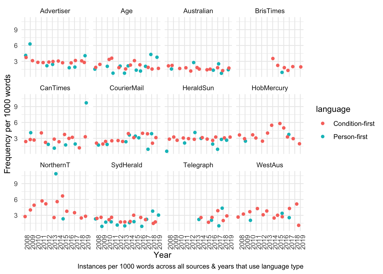
Figure 12: Visualisation of the above relative frequency per 1000 words of person-first and condition-first language by source and year.

Note that above we considered the word count ONLY in articles that featured that particular language type in the denominator

Next, we conduct the same analysis, but including all articles from that particular source, year or both (irrespective of whether they feature the language type).

Code

freq_entire_corpus <- function(df, group_vars){
  df %>%
  group_by(!!!group_vars) %>%
  summarise(
    person_first_instances = sum(person_first),
    condition_first_instances = sum(condition_first),
    total_wc = sum(wordcount_total),
    person_first_per_1000 = 1000 * person_first_instances/total_wc,
    cond_first_per_1000 = 1000 * condition_first_instances/total_wc
  )
}
condition_person_comparison_together <- 
  full_join(
    full_join(
      {person_first_annotated %>%
          select(article_id, no_hits_in_text) %>%
          rename(person_first = no_hits_in_text)},
      {condition_first_annotated %>%
          select(article_id, no_hits_in_text) %>%
          rename(condition_first = no_hits_in_text)}
    ),
    {metadata_full %>%
        select(article_id, source, year, wordcount_total)}) %>%
  # fill NAs with 0
  mutate_if(is.numeric,coalesce,0) 
  # now generate the instances
freq_entire_corpus(condition_person_comparison_together, vars(year)) %>% 
  kable()

Table 17: Number of instances of the two language types by year, total word count of articles published that year and the relative frequency of instances per 1000 words across all articles from that source.

year	person_first_instances	condition_first_instances	total_wc	person_first_per_1000	cond_first_per_1000
2008	6	553	1863018	0.0032206	0.2968302
2009	7	507	1524207	0.0045926	0.3326320
2010	4	452	1454853	0.0027494	0.3106843
2011	5	447	1318579	0.0037920	0.3390013
2012	5	385	1280045	0.0039061	0.3007707
2013	12	382	1625785	0.0073810	0.2349634
2014	9	408	1271294	0.0070794	0.3209328
2015	9	436	1596597	0.0056370	0.2730808
2016	15	388	1156387	0.0129714	0.3355278
2017	18	309	1121553	0.0160492	0.2755108
2018	9	273	1211129	0.0074311	0.2254095
2019	37	137	1012594	0.0365398	0.1352961

Code

freq_entire_corpus(condition_person_comparison_together, vars(year)) %>%
  select(year, ends_with("per_1000")) %>%
  pivot_longer(cols = ends_with("1000"), names_to = "type", values_to = "value") %>%
  mutate(type = stringr::str_replace_all(type, "_per_1000", ""),
         type = case_when(type == "cond_first" ~ "Condition-first", TRUE ~ "Person-first")) %>%
  ggplot(aes(x = as.factor(year), y= value, col = type)) +
  geom_point() + 
  labs(x = "Year",
       y = "Instances per 1000 words in corpus by year",
       col = "")

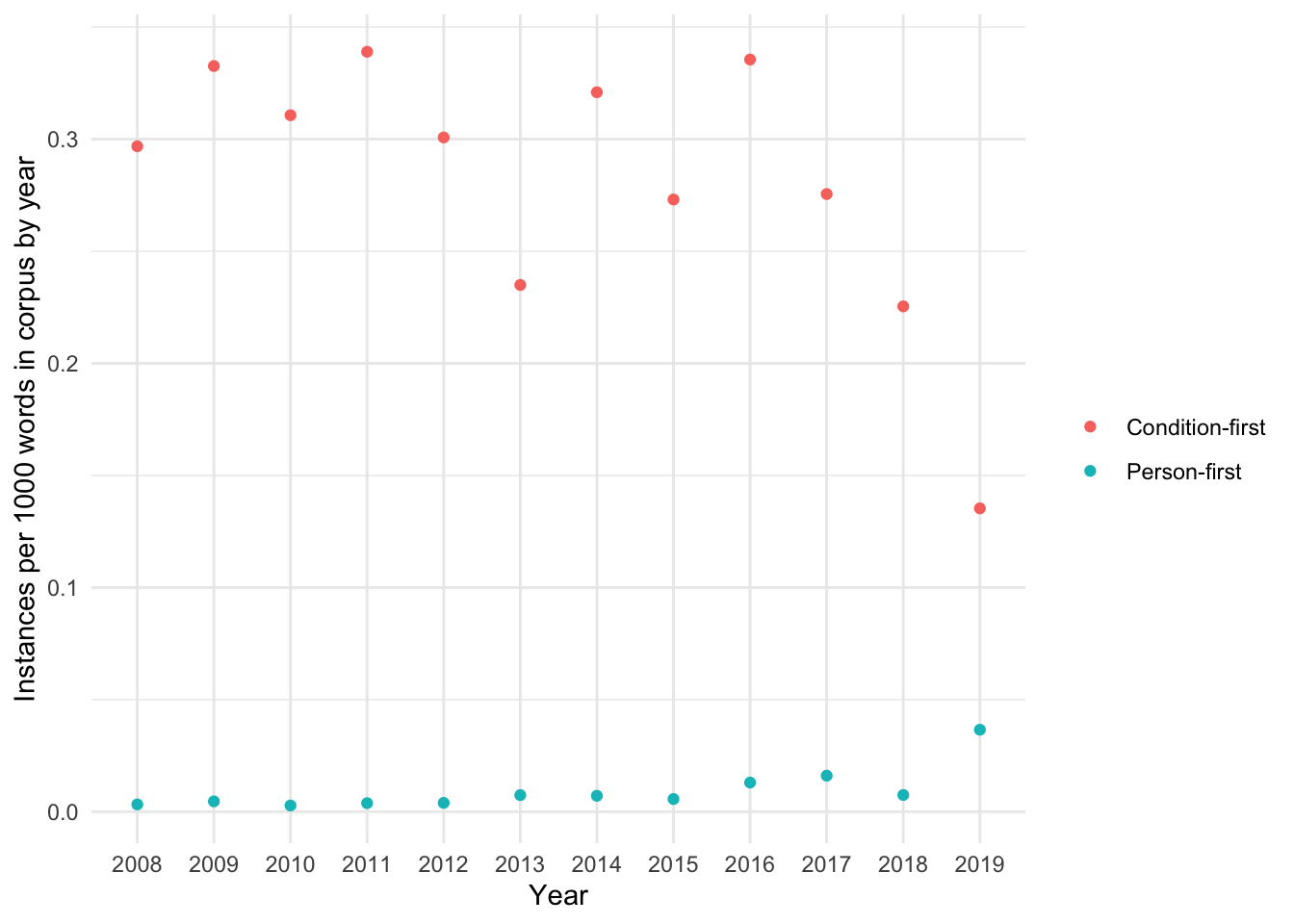
Figure 13: Visualisation of the above relative frequency per 1000 words of person-first and condition-first language by year, considering the word count of all articles in the corpus that year.

We can see that if we consider the entire corpus, instances of condition-first language seem to be somewhat lower by year in 2017 onward.

Let’s look at the numbers by source, across all years:

Code

freq_entire_corpus({condition_person_comparison_together %>% filter(!(source %in% c("Telegraph", "BrisTimes")))}, vars(source)) %>% 
  kable()

Table 18: Number of instances of the two language types by source, total word count of articles published in that source in the corpus and the relative frequency of instances per 1000 words across all articles from that source.

source	person_first_instances	condition_first_instances	total_wc	person_first_per_1000	cond_first_per_1000
Advertiser	9	636	1750948	0.0051401	0.3632318
Age	21	509	2399436	0.0087521	0.2121332
Australian	10	283	1722950	0.0058040	0.1642532
CanTimes	17	342	1431478	0.0118758	0.2389139
CourierMail	12	607	1684101	0.0071255	0.3604297
HeraldSun	16	705	1867259	0.0085687	0.3775588
HobMercury	2	240	690782	0.0028953	0.3474323
NorthernT	2	120	301923	0.0066242	0.3974523
SydHerald	37	697	2901109	0.0127537	0.2402530
WestAus	3	317	892280	0.0033622	0.3552696

Code

freq_entire_corpus({
  condition_person_comparison_together %>% 
    filter(!(source %in% c("Telegraph", "BrisTimes")))
}, vars(source)) %>%
  select(source, ends_with("per_1000")) %>%
  pivot_longer(cols = ends_with("1000"), names_to = "type", values_to = "value") %>%
  mutate(type = stringr::str_replace_all(type, "_per_1000", ""),
         type = case_when(type == "cond_first" ~ "Condition-first", TRUE ~ "Person-first")) %>%
  ggplot(aes(x = source, y= value, col = type)) +
  geom_point() + 
  labs(x = "Source",
       y = "Instances per 1000 words in corpus by source",
       col = "") +
  theme(axis.text.x = element_text(angle=90))

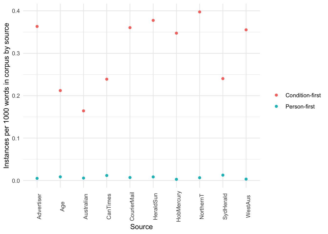
Figure 14: Visualisation of the above relative frequency per 1000 words of person-first and condition-first language by source, considering the word count of all articles in the corpus from that source.

We can see that usage of condition-first language is quite varied by source.

Let’s look at source and year simultaneously:

Code

freq_entire_corpus({condition_person_comparison_together %>% filter(!(source %in% c("Telegraph", "BrisTimes")))}, vars(source, year)) %>% 
  kable()

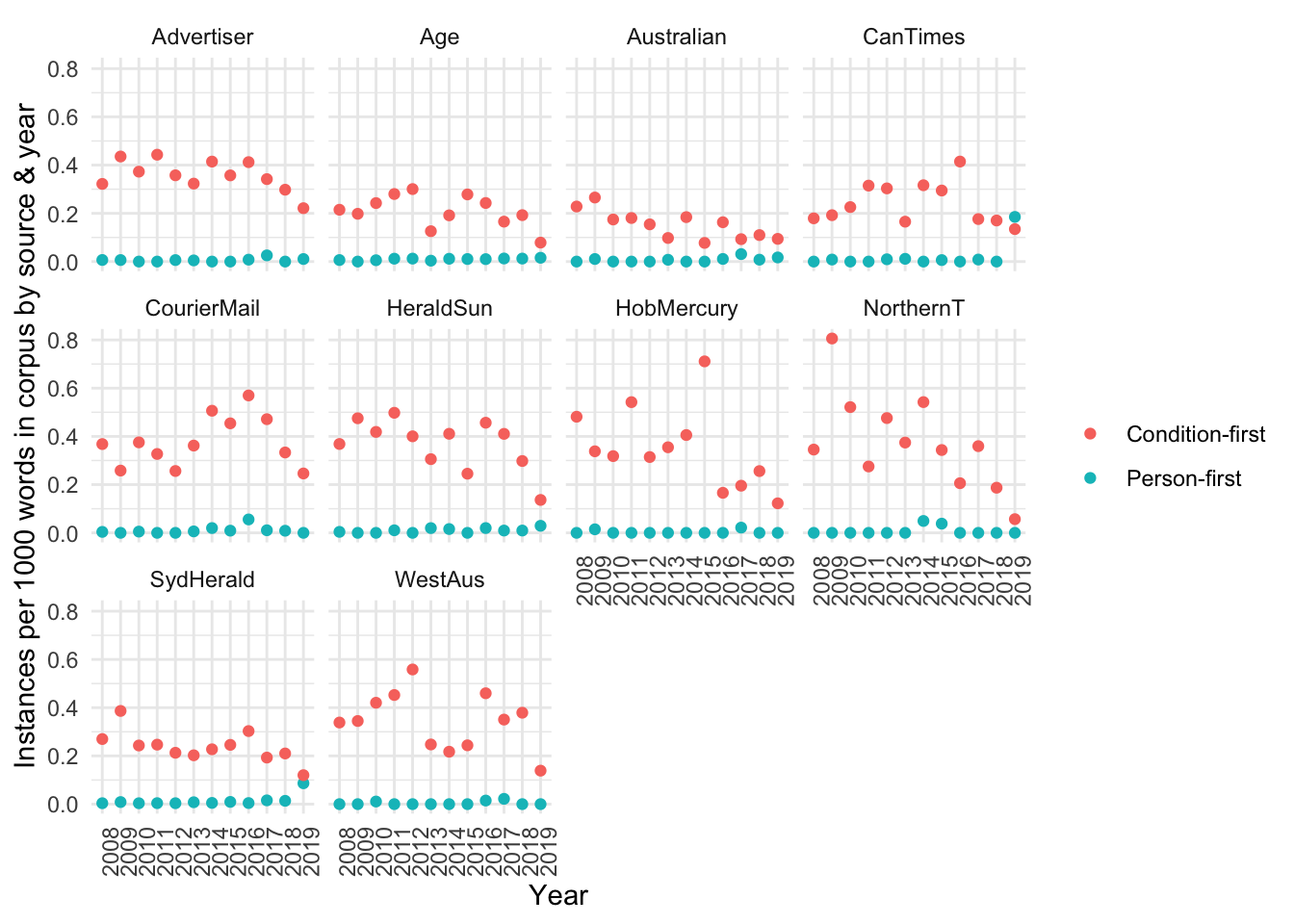
Table 19: Relative frequency per 1000 words of person-first and condition-first language by source and year, considering the word count of all articles in the corpus from that source in that year.

source	year	person_first_instances	condition_first_instances	total_wc	person_first_per_1000	cond_first_per_1000
Advertiser	2008	1	49	152154	0.0065723	0.3220421
Advertiser	2009	1	69	158395	0.0063133	0.4356198
Advertiser	2010	0	58	155561	0.0000000	0.3728441
Advertiser	2011	0	67	151211	0.0000000	0.4430895
Advertiser	2012	1	58	162157	0.0061669	0.3576781
Advertiser	2013	1	67	207306	0.0048238	0.3231937
Advertiser	2014	0	63	151973	0.0000000	0.4145473
Advertiser	2015	0	62	173493	0.0000000	0.3573631
Advertiser	2016	1	52	126129	0.0079284	0.4122763
Advertiser	2017	3	40	117002	0.0256406	0.3418745
Advertiser	2018	0	30	100696	0.0000000	0.2979264
Advertiser	2019	1	21	94871	0.0105406	0.2213532
Age	2008	2	68	316472	0.0063197	0.2148689
Age	2009	0	40	201930	0.0000000	0.1980884
Age	2010	1	44	181424	0.0055119	0.2425258
Age	2011	2	47	167790	0.0119197	0.2801120
Age	2012	2	49	163014	0.0122689	0.3005877
Age	2013	1	34	269995	0.0037038	0.1259283
Age	2014	2	33	172156	0.0116174	0.1916866
Age	2015	3	79	283729	0.0105735	0.2784347
Age	2016	2	48	197653	0.0101187	0.2428498
Age	2017	2	26	157039	0.0127357	0.1655640
Age	2018	2	31	161020	0.0124208	0.1925227
Age	2019	2	10	127214	0.0157215	0.0786077
Australian	2008	0	59	258517	0.0000000	0.2282248
Australian	2009	2	50	188289	0.0106220	0.2655492
Australian	2010	0	27	154723	0.0000000	0.1745054
Australian	2011	0	30	166076	0.0000000	0.1806402
Australian	2012	0	22	142596	0.0000000	0.1542820
Australian	2013	1	13	132956	0.0075213	0.0977767
Australian	2014	0	24	130256	0.0000000	0.1842525
Australian	2015	0	9	116308	0.0000000	0.0773807
Australian	2016	1	15	91995	0.0108702	0.1630523
Australian	2017	3	9	96918	0.0309540	0.0928620
Australian	2018	1	14	127452	0.0078461	0.1098453
Australian	2019	2	11	116864	0.0171139	0.0941265
CanTimes	2008	0	20	111564	0.0000000	0.1792693
CanTimes	2009	1	23	119572	0.0083632	0.1923527
CanTimes	2010	0	24	106258	0.0000000	0.2258653
CanTimes	2011	0	36	114314	0.0000000	0.3149221
CanTimes	2012	1	32	105464	0.0094819	0.3034211
CanTimes	2013	2	29	175309	0.0114084	0.1654222
CanTimes	2014	0	46	145337	0.0000000	0.3165058
CanTimes	2015	1	48	162947	0.0061370	0.2945743
CanTimes	2016	0	32	77167	0.0000000	0.4146850
CanTimes	2017	1	21	119117	0.0083951	0.1762973
CanTimes	2018	0	23	135017	0.0000000	0.1703489
CanTimes	2019	11	8	59412	0.1851478	0.1346529
CourierMail	2008	1	92	249904	0.0040015	0.3681414
CourierMail	2009	0	59	228541	0.0000000	0.2581594
CourierMail	2010	1	72	191892	0.0052113	0.3752111
CourierMail	2011	0	43	131489	0.0000000	0.3270236
CourierMail	2012	0	32	124784	0.0000000	0.2564431
CourierMail	2013	1	60	165817	0.0060307	0.3618447
CourierMail	2014	2	51	100723	0.0198564	0.5063392
CourierMail	2015	1	50	110106	0.0090822	0.4541079
CourierMail	2016	4	41	71961	0.0555857	0.5697531
CourierMail	2017	1	44	93348	0.0107126	0.4713545
CourierMail	2018	1	38	114008	0.0087713	0.3333099
CourierMail	2019	0	25	101528	0.0000000	0.2462375
HeraldSun	2008	1	90	244227	0.0040946	0.3685096
HeraldSun	2009	0	91	191536	0.0000000	0.4751065
HeraldSun	2010	0	82	195937	0.0000000	0.4185019
HeraldSun	2011	2	94	188824	0.0105919	0.4978181
HeraldSun	2012	0	65	162385	0.0000000	0.4002833
HeraldSun	2013	4	62	202876	0.0197165	0.3056054
HeraldSun	2014	2	52	126605	0.0157972	0.4107263
HeraldSun	2015	0	35	142687	0.0000000	0.2452921
HeraldSun	2016	2	46	100735	0.0198541	0.4566437
HeraldSun	2017	1	43	104785	0.0095434	0.4103641
HeraldSun	2018	1	31	104080	0.0096080	0.2978478
HeraldSun	2019	3	14	102582	0.0292449	0.1364762
HobMercury	2008	0	45	93465	0.0000000	0.4814636
HobMercury	2009	1	23	68016	0.0147024	0.3381557
HobMercury	2010	0	23	72280	0.0000000	0.3182070
HobMercury	2011	0	26	47973	0.0000000	0.5419715
HobMercury	2012	0	19	60444	0.0000000	0.3143405
HobMercury	2013	0	31	87371	0.0000000	0.3548088
HobMercury	2014	0	12	29587	0.0000000	0.4055835
HobMercury	2015	0	24	33753	0.0000000	0.7110479
HobMercury	2016	0	10	60253	0.0000000	0.1659668
HobMercury	2017	1	9	46038	0.0217212	0.1954907
HobMercury	2018	0	13	50759	0.0000000	0.2561122
HobMercury	2019	0	5	40843	0.0000000	0.1224200
NorthernT	2008	0	12	34752	0.0000000	0.3453039
NorthernT	2009	0	27	33503	0.0000000	0.8058980
NorthernT	2010	0	17	32606	0.0000000	0.5213764
NorthernT	2011	0	6	21798	0.0000000	0.2752546
NorthernT	2012	0	10	21011	0.0000000	0.4759412
NorthernT	2013	0	10	26708	0.0000000	0.3744196
NorthernT	2014	1	11	20290	0.0492854	0.5421390
NorthernT	2015	1	9	26207	0.0381577	0.3434197
NorthernT	2016	0	6	29146	0.0000000	0.2058602
NorthernT	2017	0	8	22253	0.0000000	0.3595021
NorthernT	2018	0	3	16032	0.0000000	0.1871257
NorthernT	2019	0	1	17617	0.0000000	0.0567634
SydHerald	2008	1	71	263075	0.0038012	0.2698850
SydHerald	2009	2	90	232899	0.0085874	0.3864336
SydHerald	2010	1	66	271396	0.0036847	0.2431871
SydHerald	2011	1	61	247334	0.0040431	0.2466301
SydHerald	2012	1	56	262970	0.0038027	0.2129520
SydHerald	2013	2	52	256756	0.0077895	0.2025269
SydHerald	2014	1	45	197915	0.0050527	0.2273703
SydHerald	2015	3	80	325532	0.0092157	0.2457516
SydHerald	2016	1	68	224438	0.0044556	0.3029790
SydHerald	2017	3	37	191646	0.0156539	0.1930643
SydHerald	2018	3	46	219004	0.0136984	0.2100418
SydHerald	2019	18	25	208144	0.0864786	0.1201092
WestAus	2008	0	47	138888	0.0000000	0.3384022
WestAus	2009	0	35	101526	0.0000000	0.3447393
WestAus	2010	1	39	92776	0.0107786	0.4203673
WestAus	2011	0	37	81770	0.0000000	0.4524887
WestAus	2012	0	42	75220	0.0000000	0.5583621
WestAus	2013	0	24	97018	0.0000000	0.2473768
WestAus	2014	0	21	96631	0.0000000	0.2173216
WestAus	2015	0	17	69706	0.0000000	0.2438814
WestAus	2016	1	31	67430	0.0148302	0.4597360
WestAus	2017	1	16	45643	0.0219092	0.3505466
WestAus	2018	0	7	18468	0.0000000	0.3790340
WestAus	2019	0	1	7204	0.0000000	0.1388118

Code

freq_entire_corpus({
  condition_person_comparison_together %>% filter(!(source %in% c("Telegraph", "BrisTimes")))
}, vars(source, year)) %>%
  select(source, year, ends_with("per_1000")) %>%
  pivot_longer(cols = ends_with("1000"), names_to = "type", values_to = "value") %>%
  mutate(type = stringr::str_replace_all(type, "_per_1000", ""),
         type = case_when(type == "cond_first" ~ "Condition-first", TRUE ~ "Person-first")) %>%
  ggplot(aes(x = as.factor(year), y= value, col = type)) +
  geom_point() + 
  facet_wrap(~source) +
  labs(x = "Year",
       y = "Instances per 1000 words in corpus by source & year",
       col = "") +
  theme(axis.text.x = element_text(angle=90))

Figure 15: Visualisation of the above relative frequency per 1000 words of person-first and condition-first language by source and year, considering the word count of all articles in the corpus from that source in that year.

Condition-first language use

We can investigate the prevalence of condition-first language using goodness of fit tests, comparing their distribution in:

• tabloids vs broadsheets
• left and right leaning publications

We can do this by looking at:

• the total number of instances in the subcorpus
• the number of articles that feature this language type

Tabloids vs broadsheets

The total number of uses of condition-first language we observe is higher in tabloids and lower in broadsheets than we would expect based on the word count in these subcorpora (p < 0.001).

Code

chisq_instances_wc_normalised(condition_first_annotated, metadata_full, source_type) |> kable()

Table 20: Results of goodness of fit test of the number of uses of condition-first language we observe in tabloids and broadsheets relative to the total word count across these two types of sources.

variable	value
method	Chi-squared test for given probabilities
parameter	1
statistic	308.1251
p.value	5.593314e-69
broadsheet_observed	1866
broadsheet_expected	2465.34566596664
tabloid_observed	2811
tabloid_expected	2211.65433403336

The number of articles with condition-first language we observe is also higher in tabloids and lower in broadsheets than we would expect based on the total article count in these subcorpora (p < 0.001).

Code

chisq_articles_totalart_normalised(condition_first_annotated, metadata_full, source_type) |> kable()

Table 21: Results of goodness of fit test of the number of articles that use condition-first language we observe in tabloids and broadsheets relative to the total word count across these two types of sources.

variable	value
method	Chi-squared test for given probabilities
parameter	1
statistic	25.73612
p.value	3.914328e-07
broadsheet_observed	1170
broadsheet_expected	1311.25451974162
tabloid_observed	2038
tabloid_expected	1896.74548025838

Left vs right-leaning publications

The total number of uses of condition-first language we observe is higher in right and lower in left-leaning publications than we would expect based on the word count in these subcorpora (p < 0.001).

Code

chisq_instances_wc_normalised(condition_first_annotated, metadata_full, orientation) |> kable()

Table 22: Results of goodness of fit test of the number of uses of condition-first language we observe in right and left leaning publications relative to the total word count across these two types.

variable	value
method	Chi-squared test for given probabilities
parameter	1
statistic	134.72
p.value	3.801809e-31
left_observed	1583
left_expected	1975.0671889295
right_observed	3094
right_expected	2701.9328110705

The number of articles with condition-first language we observe is also is higher in right and lower in left-leaning publications than we would expect based on the total article count in these subcorpora (p < 0.001).

Code

chisq_articles_totalart_normalised(condition_first_annotated, metadata_full, orientation) |> kable()

Table 23: Results of goodness of fit test of the number of articles that use condition-first language we observe in left and right leaning publications relative to the total word count across these two types.

variable	value
method	Chi-squared test for given probabilities
parameter	1
statistic	11.84526
p.value	0.0005780843
left_observed	979
left_expected	1070.92734013683
right_observed	2229
right_expected	2137.07265986317

Person-first language use

Tabloids vs broadsheets

The total number of uses of person-first language we observe is somewhat higher in tabloids and lower in broadsheets than we would expect based on the word count in these subcorpora, but this result is not strongly significant (p < 0.05).

Code

chisq_instances_wc_normalised(person_first_annotated, metadata_full, source_type) |> kable()

Table 24: Results of goodness of fit test of the number of uses of person-first language we observe in tabloids and broadsheets relative to the total word count across these two types of sources.

variable	value
method	Chi-squared test for given probabilities
parameter	1
statistic	6.041885
p.value	0.01397036
broadsheet_observed	86
broadsheet_expected	71.6884777788033
tabloid_observed	50
tabloid_expected	64.3115222211967

The number of articles with person-first language we observe is, in contrast, lower in tabloids and higher in broadsheets than we would expect based on the total article count in these subcorpora (p < 0.002).

Code

chisq_articles_totalart_normalised(person_first_annotated, metadata_full, source_type) |> kable()

Table 25: Results of goodness of fit test of the number of articles that use person-first language we observe in tabloids and broadsheets relative to the total word count across these two types of sources.

variable	value
method	Chi-squared test for given probabilities
parameter	1
statistic	9.588964
p.value	0.001957503
broadsheet_observed	59
broadsheet_expected	43.3269884952032
tabloid_observed	47
tabloid_expected	62.6730115047968

Left vs right-leaning publications

The total number of uses of person-first language we observe is higher in left and lower in right-leaning publications than we would expect based on the word count in these subcorpora (p < 0.002).

Code

chisq_instances_wc_normalised(person_first_annotated, metadata_full, orientation) |> kable()

Table 26: Results of goodness of fit test of the number of uses of person-first language we observe in right and left leaning publications relative to the total word count across these two types.

variable	value
method	Chi-squared test for given probabilities
parameter	1
statistic	10.39137
p.value	0.001266055
left_observed	76
left_expected	57.4319302318606
right_observed	60
right_expected	78.5680697681394

The number of articles with person-first language we observe is also is higher in left and lower in right-leaning publications than we would expect based on the total article count in these subcorpora (p < 0.002).

Code

chisq_articles_totalart_normalised(person_first_annotated, metadata_full, orientation) |> kable()

Table 27: Results of goodness of fit test of the number of articles that use person-first language we observe in left and right leaning publications relative to the total word count across these two types.

variable	value
method	Chi-squared test for given probabilities
parameter	1
statistic	10.34217
p.value	0.00130025
left_observed	51
left_expected	35.3860031341972
right_observed	55
right_expected	70.6139968658029

Condition-first language across time

As we discussed, we have sufficient data to explore the use of condition-first language across time and by type of publication, except for the Brisbane Times and Daily Telegraph, for which we are missing data from 2008-2013:

Code

assess_year_source(condition_first_annotated)

Table 28: Number of articles that use condition-first language by year and source.

source	2008	2009	2010	2011	2012	2013	2014	2015	2016	2017	2018	2019	Total
Advertiser	40	53	43	49	40	51	43	41	37	25	19	15	456
Age	49	24	24	28	37	25	22	34	26	18	19	9	315
Australian	35	26	20	22	17	11	16	8	9	7	12	8	191
CanTimes	15	18	14	18	24	17	31	24	18	10	19	4	212
CourierMail	65	44	50	31	25	40	38	36	29	29	28	19	434
HeraldSun	66	71	56	61	51	49	35	25	32	28	22	13	509
HobMercury	31	16	15	20	14	23	8	13	8	8	11	5	172
NorthernT	12	21	13	5	7	10	7	5	4	7	3	1	95
SydHerald	47	52	41	35	38	41	30	37	36	23	32	18	430
WestAus	38	23	28	26	36	16	17	14	17	9	3	1	228
BrisTimes	0	0	0	0	0	0	3	5	2	2	5	5	22
Telegraph	0	0	0	0	0	0	33	14	30	35	23	9	144
Total	398	348	304	295	289	283	283	256	248	201	196	107	3208

Code

condition_first_annotated_for_modelling <- condition_first_annotated %>%
  filter( !(source %in% c("BrisTimes", "Telegraph")))

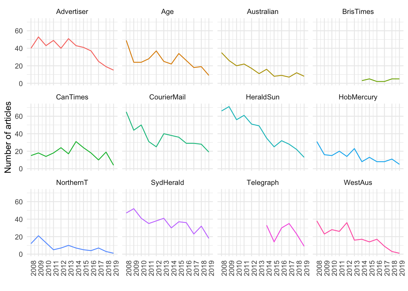
Let’s look at the number of articles by publication and year. We can see that this number is declining; however, this is likely to be attributable to the overall decline in the number of articles featuring obes*, as discussed in the exploratory data analysis section

Code

condition_first_annotated %>%
  select(year, source, source_type) %>%
  group_by(year, source) %>%
  count() %>%
  ggplot(aes(x = year, y = n, col = source)) + 
  geom_line() +
  labs(x = "", y = "Number of articles") +
  theme(axis.text.x = element_text(angle = 90),
        legend.position = "NA") +
  scale_x_continuous(breaks = unique(condition_first_annotated$year)) + 
  facet_wrap(~source)

Figure 16: Line plot of the number of articles that use condition-first language by year and source.

Normalised frequency

The normalised frequency is distributed log-normally across all texts:

Code

condition_first_annotated %>%
  select(frequency) %>%
  ggplot(aes(x = log(frequency))) + 
  geom_histogram(bins = 75)

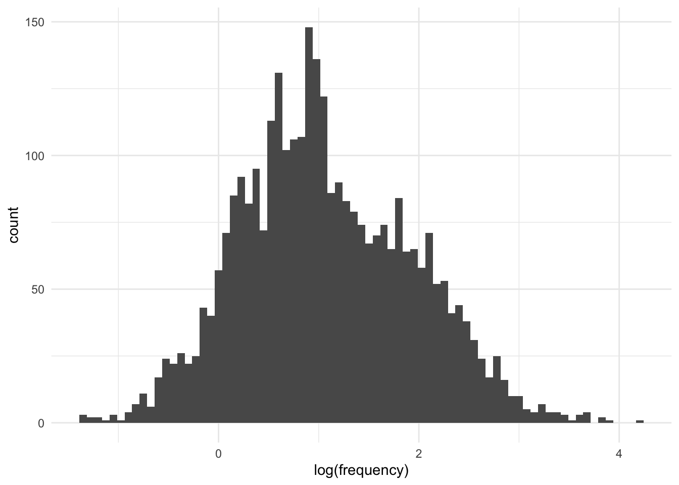
Figure 17: Histogram of the natural logarithm of the normalised frequency of condition-first language across all articles.

Let’s look at the difference in frequency across time (only the variability of which should be sensitive to the number of articles per year, not the absolute values):

We can start by using a jitter plot:

Code

condition_first_annotated %>%
  ggplot(aes(x = as.factor(year), 
             y = log(frequency), 
             fill = year)) + 
  geom_jitter(alpha = 0.2) +
  geom_smooth(aes(group = source), col = "blue", method = "loess") +
  geom_hline(yintercept = 1, col = "red", lty = 3) + 
  facet_wrap(~source) + 
  theme(axis.text.x = 
          element_text(angle = 90, vjust = 0.5, hjust=1),
        legend.position = "NA") + 
  labs(
    x = "Year",
    y = "log(frequency per 1000 words)"
  )

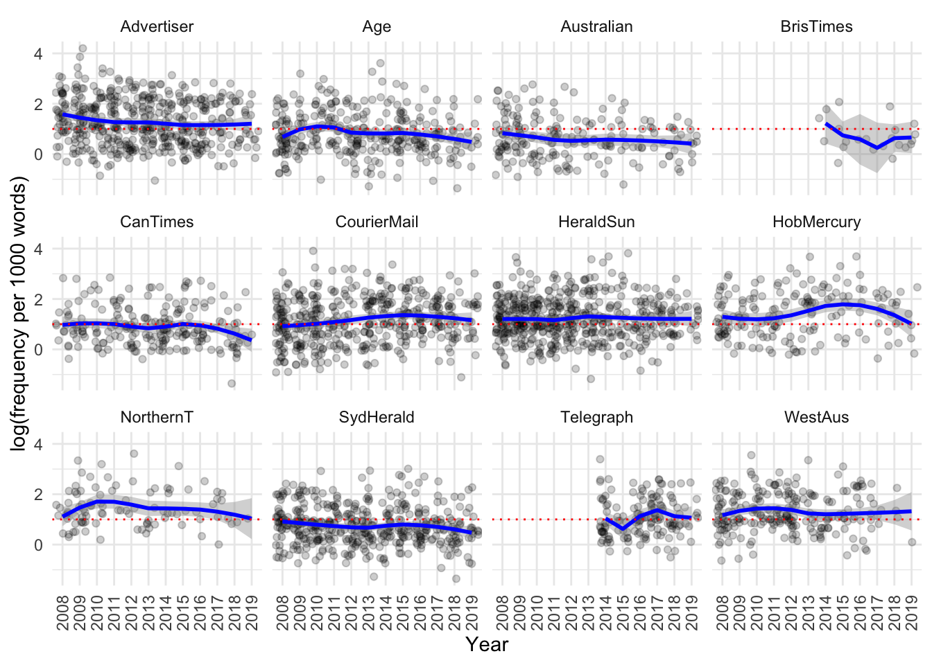
Figure 18: Jitter plot of raw values and loess smoothing (blue line) of natural logarithm of normalised frequency of condition-first language by year for each source.

Note that the dashed red line is always at the same position (with a value of exp(1) = 2.72). Comparing it with the blue line of best fit for each source for which we have complete data suggests that visually we cannot discern strong trends in the use of condition-first language across the study time period, so using variability-based neighbor clustering (VNC) is unlikely to provide meaningful results for this research question.

We can see that the Advertiser seems to have higher median frequencies than others, as does the Northern Territorian. Let’s look at it grouped as tabloid vs broadsheet (with outliers not shown):

Code

condition_first_annotated %>%
  select(year, source, source_type, frequency) %>%
  mutate(year = as.factor(year)) %>%
  group_by(year, source_type) %>%
  ggplot(aes(x = year, y = frequency, fill = source_type)) +
  geom_boxplot(outlier.shape = NA) +
  coord_cartesian(ylim = quantile(condition_first_annotated$frequency, c(0.05, 0.95))) +
  labs(
    x = "",
    y = "Frequency per thousand words",
    fill = "Source type"
  )

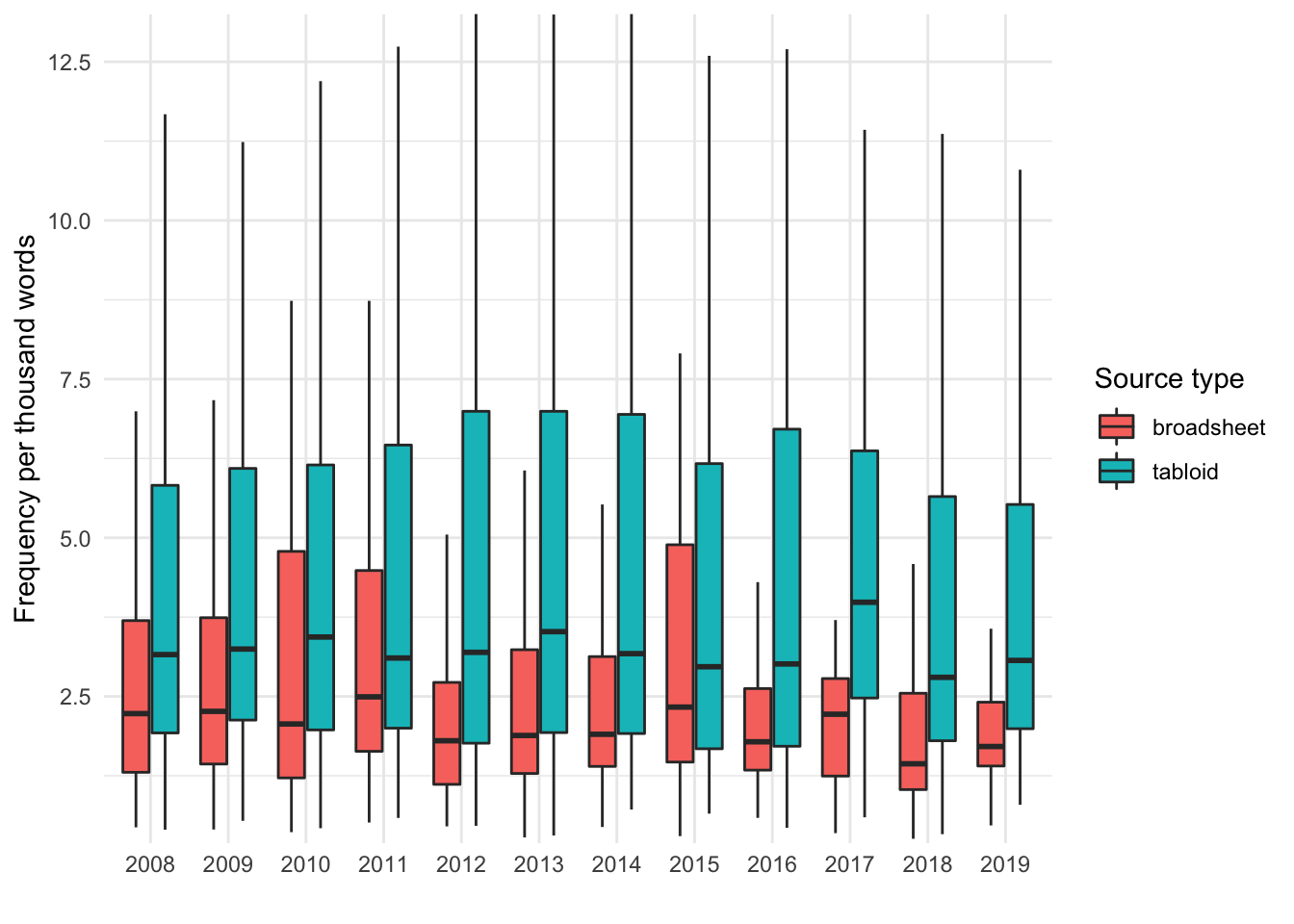
Figure 19: Boxplot of the frequency of condition-first language by year across tabloids and broadsheets, with outliers not shown.

It appears that median frequency in tabloids is somewhat higher, although the intervals do overlap across all years.

Code

condition_first_annotated %>%
  ggplot(aes(x = as.factor(year), 
             y = log(frequency), 
             fill = year)) + 
  geom_jitter(alpha = 0.2) +
  geom_smooth(aes(group = source_type), col = "blue", method = "lm") +
  geom_hline(yintercept = 1, col = "red", lty = 3) + 
  facet_wrap(~source_type) + 
  theme(axis.text.x = 
          element_text(angle = 90, vjust = 0.5, hjust=1),
        legend.position = "NA") + 
  labs(
    x = "Year",
    y = "log(frequency per 1000 words)"
  )

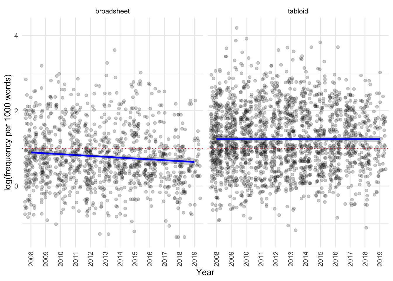
Figure 20: Jitter plot of natural logarithm of frequency of condition first language per 1000 words by year, split across tabloids and broadsheets, with blue line showing linear trend.

We can see that the frequency seems to decrease in broadsheets but not in tabloids across years.

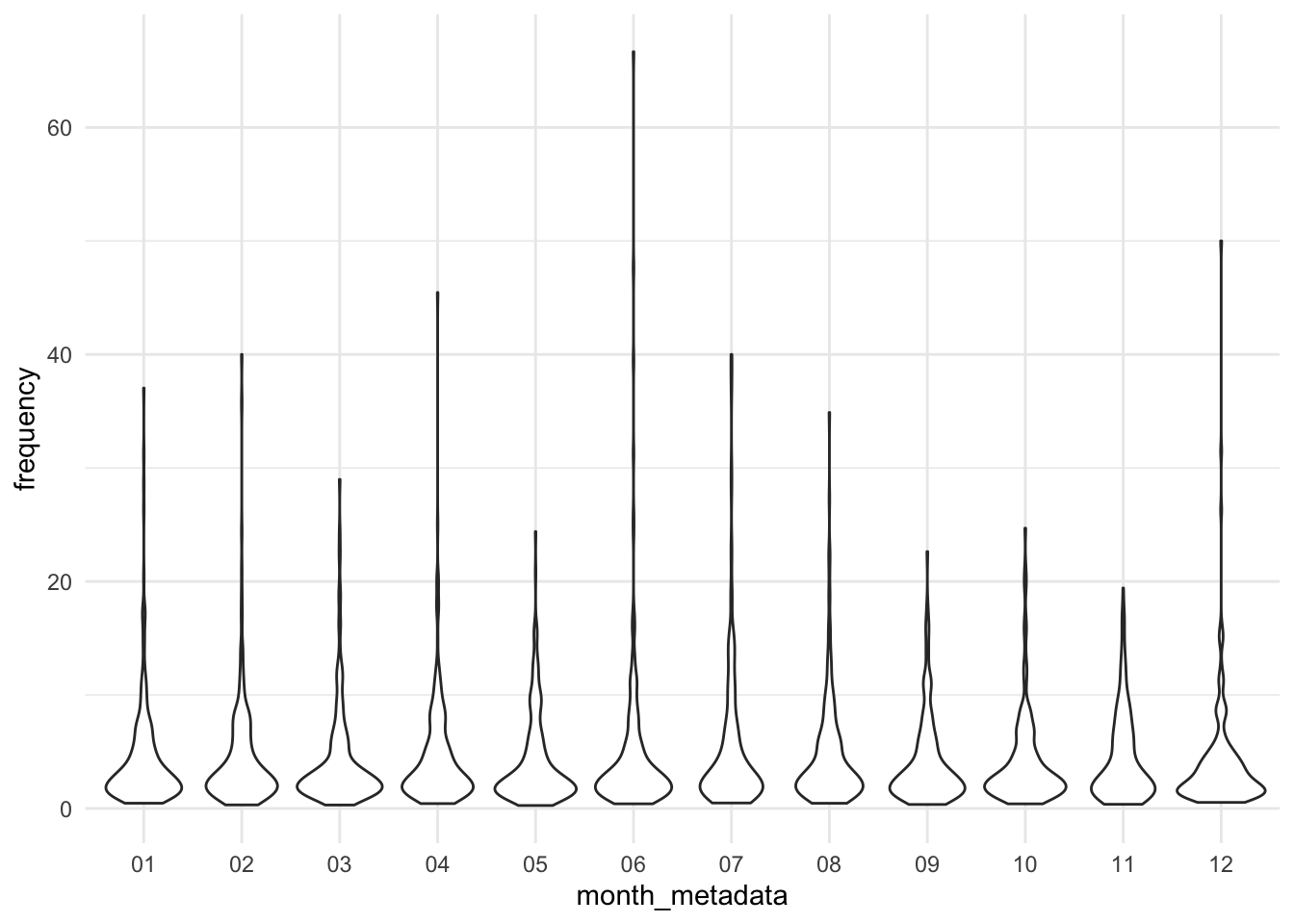
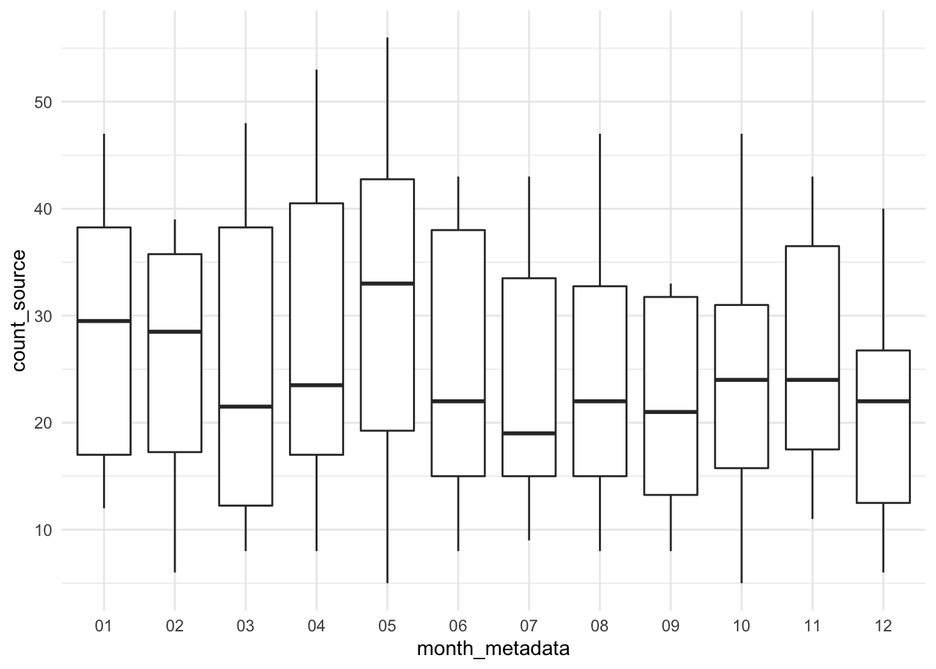
Let’s quickly look at differences by month:

Code

condition_first_annotated_for_modelling %>% 
  select(month_metadata, source, frequency) %>%
  ggplot(aes(y = frequency, x = month_metadata)) + 
  geom_violin()

Figure 21: Violin plot of frequency of condition-first language by month.

The frequency doesn’t seem to be different month to month, when visualised using a violin or box plots.

Code

condition_first_annotated_for_modelling %>% 
  select(month_metadata, source) %>%
  group_by(month_metadata, source) %>%
  mutate(count_source = n()) %>%
  distinct() %>%
  ungroup() %>%
  ggplot(aes(y = count_source, x = month_metadata)) +
  geom_boxplot()

Figure 22: Boxplot of frequency of condition-first language by month.

Condition-first language - modelling frequency

We will use a linear mixed effects model to consider whether there are differences in the frequency of condition-first language use in broadsheets and tabloids across years, including whether there are differences in specific publications. We will also use simple linear models to explore

When constructing the model we will:

• Use log(frequency) as the dependent variable, as this is normally distributed
• Center and scale the date

Code

condition_first_annotated_for_modelling$scaled_year <- scale(condition_first_annotated_for_modelling$year, scale = F)
library(broom.mixed)
# base model
m_0_base <- glm(log(frequency) ~ 1, family = gaussian, 
                data = condition_first_annotated_for_modelling)
# with year
m_0_year <- glm(log(frequency) ~ scaled_year, family = gaussian, 
                data = condition_first_annotated_for_modelling)
# with year and source type
m_0_yearsourcetype <- glm(log(frequency) ~ scaled_year + source_type, family = gaussian, 
                data = condition_first_annotated_for_modelling)
# with year and source type
m_0_yearsource <- glm(log(frequency) ~ scaled_year + source, family = gaussian, 
                data = condition_first_annotated_for_modelling)
# with source
m_0_source = lmer(log(frequency) ~ 1 + (1|source), REML = T, 
                  data = condition_first_annotated_for_modelling)

Does including a random intercept for each source improve our model?

Code

rbind(
  {glance(m_0_base) %>% mutate(model = "Base") %>% dplyr::select(-df.null, -null.deviance, -deviance)},
  {glance(m_0_year) %>% mutate(model = "With year") %>% dplyr::select(-df.null, -null.deviance, -deviance)},
  {glance(m_0_yearsourcetype) %>% mutate(model = "With year & source type") %>% dplyr::select(-df.null, -null.deviance, -deviance)},
  {glance(m_0_yearsource) %>% mutate(model = "With year & source") %>% dplyr::select(-df.null, -null.deviance, -deviance)},
  {glance(m_0_source) %>% mutate(model = "With source") %>% dplyr::select(-sigma, -REMLcrit)}
) %>% 
  arrange(AIC) %>%
  kable()

Table 29: Log-likelihood, Akaike Information Criterion (AIC), Bayesian Information Criterion (BIC), residual number of degrees of freedom and number of observations used to fit a range of general linear models.

logLik	AIC	BIC	df.residual	nobs	model
-3749.974	7523.948	7596.191	3031	3042	With year & source
-3766.832	7541.663	7565.744	3039	3042	With year & source type
-3774.515	7555.030	7573.091	3039	3042	With source
-3876.393	7758.785	7776.846	3040	3042	With year
-3878.926	7761.851	7773.892	3041	3042	Base

Yes, it seems that the AIC and BIC are reduced while the logLik is higher for the model that includes source and year. So, yes, it seems using a random effects model for source may be an option.

Now let’s build several different random effects models:

• Including year as a fixed effect
• Including each specific source (random effect) individually and year

Code

#library(afex)
m_1_base <- lmer(log(frequency) ~ 1 + (1|source), 
                 data = condition_first_annotated_for_modelling,
                 REML = FALSE, 
                 control = lmerControl(optimizer ='optimx', optCtrl=list(method='nlminb')))
# random intercept for each source
m_1_year <- lmer(log(frequency) ~ scaled_year + (1|source), 
                 data = condition_first_annotated_for_modelling,
                 REML = FALSE, 
                 control = lmerControl(optimizer ='optimx', optCtrl=list(method='nlminb')))
# random intercept for each source
m_1_year_sourcetype <- lmer(log(frequency) ~ scaled_year + source_type +(1|source), 
                 data = condition_first_annotated_for_modelling,
                 REML = FALSE, 
                 control = lmerControl(optimizer ='optimx', optCtrl=list(method='nlminb')))
# random slope and intercept for each source
m_1_yearsource <- lmer(log(frequency) ~ scaled_year + (scaled_year|source), 
                 data = condition_first_annotated_for_modelling,
                 REML = FALSE, 
                 control = lmerControl(optimizer ='optimx', optCtrl=list(method='nlminb')))
# random slope and intercept for each source
m_1_full <- lmer(log(frequency) ~ scaled_year + source_type + (scaled_year|source), 
                 data = condition_first_annotated_for_modelling,
                 REML = FALSE, 
                 control = lmerControl(optimizer ='optimx', optCtrl=list(method='nlminb')))
# random intercept for each source type
m_1_year_sourcetype_nosource <- 
  lmer(log(frequency) ~ scaled_year +(1|source_type), 
                 data = condition_first_annotated_for_modelling,
                 REML = FALSE, 
                 control = lmerControl(optimizer ='optimx', optCtrl=list(method='nlminb')))
# use the all_fit function to assess which optimisers work
#all_fit(m_1_yearsource)
# m_1_yearsource_apex <- 
#   mixed(log(frequency) ~ scaled_year + (scaled_year|source), 
#       data = condition_first_annotated_for_modelling,
#       method = "PB",
#       REML=FALSE,
#       control = lmerControl(optimizer ='optimx', optCtrl=list(method='nlminb')))
# m_1_yearsource_apex

We end up needing to use the nlminb optimiser from the optimx library (originally used by lme4), as the default REML fails to converge for the most complex model.

Code

purrr::map_dfr(list(
  m_1_base,
  m_1_year,
  m_1_year_sourcetype,
  m_1_yearsource,
  m_1_year_sourcetype_nosource,
  m_1_full),
        ~(glance(.x))) %>%
  mutate(model = c(
    "1 + (1|source)",
    "scaled_year + (1|source)",
    "scaled_year + source_type +(1|source)",
    "scaled_year + (scaled_year|source)",
    "scaled_year + (1|sourcetype)",
    "scaled_year + source_type + (scaled_year|source)"
  )) %>%
  arrange(AIC) %>%
  kable()

Table 30: Log-likelihood, Akaike Information Criterion (AIC), Bayesian Information Criterion (BIC), residual number of degrees of freedom and number of observations used to fit a range of random effects models.

nobs	sigma	logLik	AIC	BIC	deviance	df.residual	model
3042	0.8284958	-3755.568	7525.136	7567.277	7511.136	3035	scaled_year + source_type + (scaled_year|source)
3042	0.8315654	-3761.807	7533.613	7563.715	7523.613	3037	scaled_year + source_type +(1|source)
3042	0.8281507	-3764.163	7540.327	7576.448	7528.327	3036	scaled_year + (scaled_year|source)
3042	0.8314829	-3771.826	7551.651	7575.732	7543.651	3038	scaled_year + (1|source)
3042	0.8317932	-3773.010	7552.021	7570.082	7546.021	3039	1 + (1|source)
3042	0.8349904	-3772.598	7553.197	7577.278	7545.197	3038	scaled_year + (1|sourcetype)

The full model (scaled_year + source_type + (scaled_year|source)) has the lowest AIC and highest log-Likelihood among the mixed effects models. However, it’s AIC is not that different (7524 vs 7525) to the simpler model scaled_year + source, while the simpler model has a lower BIC and higher logLik.

Let’s compare the two models: the full mixed effects model and the simple scaled_year + source

Code

anova(m_1_full, m_0_yearsource)

Data: condition_first_annotated_for_modelling
Models:
m_1_full: log(frequency) ~ scaled_year + source_type + (scaled_year | source)
m_0_yearsource: log(frequency) ~ scaled_year + source
               npar    AIC    BIC  logLik deviance  Chisq Df Pr(>Chisq)  
m_1_full          7 7525.1 7567.3 -3755.6   7511.1                       
m_0_yearsource   12 7523.9 7596.2 -3750.0   7499.9 11.188  5    0.04778 *
---
Signif. codes:  0 '***' 0.001 '**' 0.01 '*' 0.05 '.' 0.1 ' ' 1

It seems that the more complex model does not offer a substantial improvement in fit over the simpler one. Let’s summarise that model.

Code

report::report(m_0_yearsource)

‘r2()’ does not support models of class ‘glm’. ‘r2()’ does not support models of class ‘glm’. We fitted a linear model (estimated using ML) to predict frequency with scaled_year and source (formula: log(frequency) ~ scaled_year + source). . The model’s intercept, corresponding to scaled_year = 0 and source = Advertiser, is at 1.28 (95% CI [1.21, 1.36], t(3031) = 32.98, p < .001). Within this model:

• The effect of scaled year is statistically non-significant and negative (beta = -7.05e-03, 95% CI [-0.02, 2.13e-03], t(3031) = -1.50, p = 0.132; Std. beta = -9.82e-03, 95% CI [-0.02, 3.54e-03])
• The effect of source [Age] is statistically significant and negative (beta = -0.45, 95% CI [-0.57, -0.33], t(3031) = -7.43, p < .001; Std. beta = -0.19, 95% CI [-0.25, -0.14])
• The effect of source [Australian] is statistically significant and negative (beta = -0.65, 95% CI [-0.79, -0.51], t(3031) = -9.12, p < .001; Std. beta = -0.27, 95% CI [-0.33, -0.21])
• The effect of source [CanTimes] is statistically significant and negative (beta = -0.37, 95% CI [-0.50, -0.23], t(3031) = -5.33, p < .001; Std. beta = -0.18, 95% CI [-0.24, -0.12])
• The effect of source [CourierMail] is statistically significant and negative (beta = -0.14, 95% CI [-0.25, -0.03], t(3031) = -2.48, p = 0.013; Std. beta = -0.07, 95% CI [-0.12, -0.02])
• The effect of source [HeraldSun] is statistically non-significant and negative (beta = -0.06, 95% CI [-0.17, 0.04], t(3031) = -1.18, p = 0.240; Std. beta = -0.05, 95% CI [-0.09, -2.66e-04])
• The effect of source [HobMercury] is statistically non-significant and positive (beta = 0.13, 95% CI [-0.02, 0.27], t(3031) = 1.68, p = 0.092; Std. beta = 0.05, 95% CI [-0.01, 0.12])
• The effect of source [NorthernT] is statistically non-significant and positive (beta = 0.16, 95% CI [-0.02, 0.35], t(3031) = 1.72, p = 0.086; Std. beta = 0.04, 95% CI [-0.04, 0.12])
• The effect of source [SydHerald] is statistically significant and negative (beta = -0.53, 95% CI [-0.64, -0.42], t(3031) = -9.42, p < .001; Std. beta = -0.23, 95% CI [-0.28, -0.19])
• The effect of source [WestAus] is statistically non-significant and positive (beta = 0.02, 95% CI [-0.12, 0.15], t(3031) = 0.24, p = 0.808; Std. beta = -0.02, 95% CI [-0.08, 0.04])

Standardized parameters were obtained by fitting the model on a standardized version of the dataset. 95% Confidence Intervals (CIs) and p-values were computed using

If we use the BIC as our model selection criteria instead, the model of the form has the lowest BIC:

Code

purrr::map_dfr(list(
  m_1_base,
  m_1_year,
  m_1_year_sourcetype,
  m_1_yearsource,
  m_1_year_sourcetype_nosource,
  m_1_full),
        ~(glance(.x))) %>%
  mutate(model = c(
    "1 + (1|source)",
    "scaled_year + (1|source)",
    "scaled_year + source_type +(1|source)",
    "scaled_year + (scaled_year|source)",
    "scaled_year + (1|sourcetype)",
    "scaled_year + source_type + (scaled_year|source)"
  )) %>%
  arrange(BIC) %>%
  kable()

Table 31: Log-likelihood, Akaike Information Criterion (AIC), Bayesian Information Criterion (BIC), residual number of degrees of freedom and number of observations used to fit a range of random effects models.

nobs	sigma	logLik	AIC	BIC	deviance	df.residual	model
3042	0.8315654	-3761.807	7533.613	7563.715	7523.613	3037	scaled_year + source_type +(1|source)
3042	0.8284958	-3755.568	7525.136	7567.277	7511.136	3035	scaled_year + source_type + (scaled_year|source)
3042	0.8317932	-3773.010	7552.021	7570.082	7546.021	3039	1 + (1|source)
3042	0.8314829	-3771.826	7551.651	7575.732	7543.651	3038	scaled_year + (1|source)
3042	0.8281507	-3764.163	7540.327	7576.448	7528.327	3036	scaled_year + (scaled_year|source)
3042	0.8349904	-3772.598	7553.197	7577.278	7545.197	3038	scaled_year + (1|sourcetype)

We obtain a result similar to that of the simpler model:

Code

report::report(m_1_year_sourcetype)

We fitted a linear mixed model (estimated using ML and optimx optimizer) to predict frequency with scaled_year and source_type (formula: log(frequency) ~ scaled_year + source_type). The model included source as random effect (formula: ~1 | source). The model’s total explanatory power is weak (conditional R2 = 0.09) and the part related to the fixed effects alone (marginal R2) is of 0.08. The model’s intercept, corresponding to scaled_year = 0 and source_type = broadsheet, is at 0.79 (95% CI [0.69, 0.88], t(3037) = 16.43, p < .001). Within this model:

• The effect of scaled year is statistically non-significant and negative (beta = -6.94e-03, 95% CI [-0.02, 2.23e-03], t(3037) = -1.48, p = 0.138; Std. beta = -9.60e-03, 95% CI [-0.02, 3.73e-03])
• The effect of source type [tabloid] is statistically significant and positive (beta = 0.50, 95% CI [0.38, 0.62], t(3037) = 8.06, p < .001; Std. beta = 0.20, 95% CI [0.16, 0.25])

Standardized parameters were obtained by fitting the model on a standardized version of the dataset. 95% Confidence Intervals (CIs) and p-values were computed using

To summarise:

• The effect of year was not found to be significant.
• Relative to the Advertiser, the Age, Australian, Canberra Times, Courier Mail and Sydney Morning Herald had less frequency of condition-first language.