Obesity phase 2 - Exploring usage of the lemma OBESE

Exploring usage of the adjective lemma OBESE

There is interest in exploring statistics around the use of the adjective lemma OBESE around the following research questions:

Do tabloids use OBESE more than broadsheets?
Or do broadsheets use OBESE more than tabloids?
Or is there no discernible pattern of use?
Is there any newspaper that uses OBESE more than others?
Any year where OBESE is the most frequent/least frequent?

Additional question:

Is there a difference of use by primary topic?

Executive summary

1. Tabloids use the adjective lemma OBESE more frequently than broadsheets.

More specifically, a Welch Two Sample t-test testing the difference between the frequency in broadsheets per 1000 words and frequency in tabloids (mean of broadsheets = 3.16, mean of tabloids = 5.59) suggests that the effect is negative, statistically significant, and small (difference = -2.43, 95% CI [-2.63, -2.23], t(10062.88) = -24.01, p < .001; Cohen’s d = -0.46, 95% CI [-0.50, -0.42]).
The total number of uses of OBESE we observe is higher in tabloids and right leaning-publications, and and lower in broadsheets and left-leaning publications than we would expect based on the word count in these subcorpora (p < 0.001).
The number of articles with use of OBESE we observe is not different between tabloids and broadsheets, or between left and right leaning publications.

2. Tabloids have shorter article lengths than broadsheets.

More specifically, using a Welch Two Sample t-test comparing the mean word count of articles from broadsheets and tabloids (mean of broadsheet = 778.84, mean of tabloid = 485.42) suggests that the effect is positive, statistically significant, and medium (difference = 293.42, 95% CI [273.82, 313.02], t(7348.69) = 29.34, p < .001; Cohen’s d = 0.60, 95% CI [0.56, 0.65])

3. Investigating the data by source and year revealed that these variables explained a small amount of variance in the data, with OBESE being used less frequently in the Age, Australian, Canberra Times and Sydney Morning Herald relative to the Advertiser, while in the Hobart Mercury and Northern Territorian it was used somewhat more frequently than in the Advertiser. Use of the adjective lemma OBESE decreased with time in the corpus.

4. Significant differences in the use of OBESE were observed in articles on different topics, with articles annotated as “Awards” and “Bio-medical Research” using more instances per 1000 words than articles discussing politics, schooling, transport and commuting.

5. Significant differences in article topics were also observed between tabloids and broadsheets, with the topics “ChildrenParents”, “NutritionStudy”, “WomenPregnancy” and “FitnessExercise” approximately 3x more frequently reported on in tabloids than broadsheets, in contrast to topics like “Politics” and “SportsDoping”, which were approximately evenly represented between the two media types.

Data source

CQPweb data was provided. To calculate normalised frequency, we divide the number of observations from CQPweb by the word count in each article as calculated in Python, and multiple by 1000.

Code

library(here)
library(janitor)
library(readr)
library(dplyr)
library(ggplot2)
library(tidyr)
library(knitr)
library(patchwork)
library(ggfortify)
theme_set(theme_minimal())

Code

source(here::here("400_analysis", "functions.R"))

Code

adj_obese <- read_cqpweb("aoc_all_obese_tagadjlemma.txt") 
metadata <- read_csv(here("100_data_raw", "corpus_cqpweb_metadata.csv"))
additional_source_metadata <- read_csv(here("100_data_raw", "addition_source_metadata.csv"))
topic_labels <- read_csv(here("100_data_raw", "topic_labels.csv"))
metadata_full <- inner_join(inner_join(metadata,
                                       topic_labels,
                                       by = c("dominant_topic" = "topic_number")),
                            additional_source_metadata)
obese_annotated <- inner_join(
  adj_obese, metadata_full, by = c("text" = "article_id")) %>% 
  mutate(frequency = 10^3*no_hits_in_text/wordcount_total)|>
  rename(article_id = text)

We group articles into tabloids and broadsheets, and by orientation, in the following manner:

Code

metadata_full |>
  select(source, source_type, orientation) |>
  distinct() |>
  kable()

Table 1: Classification of sources into types and by orientation.
source	source_type	orientation
Advertiser	tabloid	right
Australian	broadsheet	right
NorthernT	tabloid	right
CourierMail	tabloid	right
Age	broadsheet	left
SydHerald	broadsheet	left
Telegraph	tabloid	right
WestAus	tabloid	right
CanTimes	broadsheet	left
HeraldSun	tabloid	right
HobMercury	tabloid	right
BrisTimes	broadsheet	left

Tabloid vs broadsheet

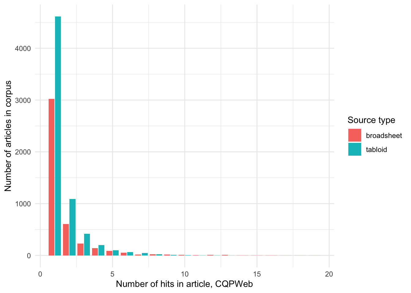
What is the distribution of OBESE in articles?

Code

obese_annotated %>%
  ggplot(aes(x = no_hits_in_text, fill = source_type)) +
  geom_bar(position = "dodge2") +
  labs(
    x = "Number of hits in article, CQPWeb",
    y = "Number of articles in corpus",
    fill = "Source type"
  )

Figure 1: Number of uses of OBESE across articles from broadsheets and tabloids.

How is this usage distributed by year (number of articles in corpus)?

Code

obese_annotated_filtered <- obese_annotated %>%
  filter(!(source %in% c("BrisTimes", "Telegraph")))
assess_year_source(obese_annotated)

Table 2: Number of articles that use OBESE by year and source.
source	2008	2009	2010	2011	2012	2013	2014	2015	2016	2017	2018	2019	Total
Advertiser	130	144	115	127	125	158	122	127	100	96	77	75	1396
Age	140	85	107	85	102	94	88	135	93	90	63	44	1126
Australian	115	84	68	76	58	47	61	33	35	34	62	36	709
CanTimes	71	85	70	79	72	88	98	88	54	77	65	26	873
CourierMail	167	144	125	110	97	118	122	108	100	85	118	74	1368
HeraldSun	196	201	171	183	138	157	121	95	84	89	95	75	1605
HobMercury	75	59	56	57	60	63	27	33	32	32	43	38	575
NorthernT	49	54	45	30	33	31	27	30	18	20	22	12	371
SydHerald	158	126	129	130	130	124	101	142	105	110	98	81	1434
WestAus	114	96	90	98	95	77	83	44	53	27	16	6	799
BrisTimes	0	0	0	0	0	1	9	37	5	7	19	22	100
Telegraph	0	0	0	0	0	0	93	52	86	95	79	60	465
Total	1215	1078	976	975	910	958	952	924	765	762	757	549	10821

We can see that apart from the Brisbane times and Daily Telegraph, there are articles using OBESE every year and in every publication. We will filter out these two sources.

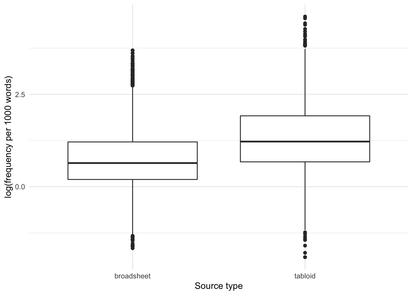
How is the frequency (per thousand words) of the usage of OBESE distributed by tabloids/broadsheets?

Code

obese_annotated_filtered %>%
  ggplot(aes(x = source_type, y = log(frequency))) + 
  geom_boxplot() + 
  labs(
    x = "Source type",
    y = "log(frequency per 1000 words)"
  )

Figure 2: Frequency per 1000 words of usage of OBESE in tabloids and broadsheets.

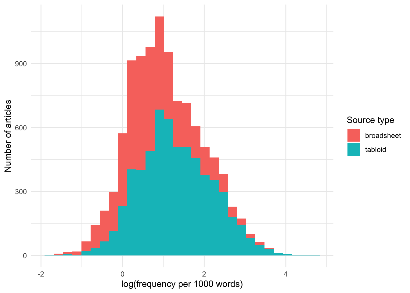
And let’s also use a histogram to look at the distribution:

Code

obese_annotated_filtered %>%
  ggplot(aes(fill = source_type,x = log(frequency))) + 
  geom_histogram() + 
  labs(
    fill = "Source type",
    x = "log(frequency per 1000 words)",
    y = "Number of articles"
  )

Figure 3: Histogram of the distribution of usage of OBESE in tabloids and broadsheets.

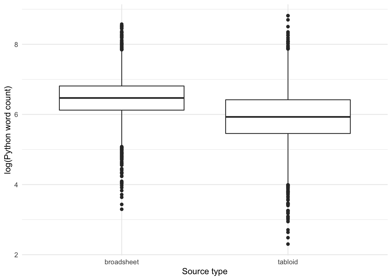
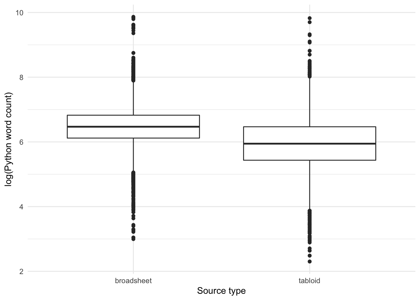
Note that broadsheets have somewhat longer texts than tabloids:

Code

obese_annotated_filtered %>%
  ggplot(aes(x = source_type, y = log(wordcount_total))) + 
  geom_boxplot() + 
  labs(
    x = "Source type",
    y = "log(Python word count)"
  )

Figure 4: Length of articles that use the lemma OBESE in tabloids and broadsheets.

Let’s use a histogram to look at the distribution in more detail:

Code

obese_annotated_filtered %>%
  ggplot(aes(fill = source_type, x = log(wordcount_total))) + 
  geom_histogram(binwidth = 0.1)+ 
  labs(
    y = "Number of articles",
    x = "log(Python word count)"
  )

Figure 5: Histogram of article lengths in tabloids and broadsheets that use the lemma OBESE.

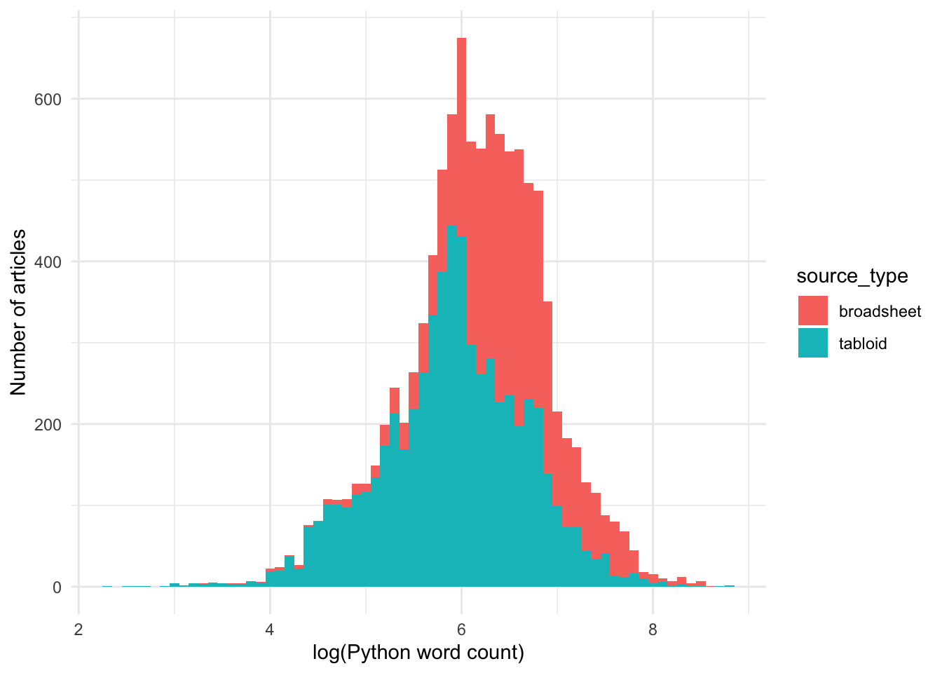
The log-transformed word count data is approximately normally distributed.

Let’s see if the difference in length of articles using the adjective lemma OBESE in tabloids and broadsheets is significant?

Code

wordcount_broadsheet <- obese_annotated_filtered[obese_annotated_filtered$source_type == "broadsheet","wordcount_total", drop = TRUE]
wordcount_tabloid <- obese_annotated_filtered[obese_annotated_filtered$source_type == "tabloid","wordcount_total", drop = TRUE]
report::report(t.test(wordcount_broadsheet,wordcount_tabloid))

The Welch Two Sample t-test testing the difference between wordcount_broadsheet and wordcount_tabloid (mean of x = 778.84, mean of y = 485.42) suggests that the effect is positive, statistically significant, and medium (difference = 293.42, 95% CI [273.82, 313.02], t(7348.69) = 29.34, p < .001; Cohen’s d = 0.60, 95% CI [0.56, 0.65])

Yes, overall articles that use the adjective lemma OBESE in tabloids are significantly shorter than in broadsheets.

This is supported by a non-parametric test as well:

Code

fp_test(wc1 = wordcount_broadsheet,
        wc2 = wordcount_tabloid,
        label1 = "broadsheet",
        label2 = "tabloid",
        dist = mydistribution)


    Approximative Two-Sample Fisher-Pitman Permutation Test
data:  wc by label (broadsheet, tabloid)
Z = 29.474, p-value < 1e-04
alternative hypothesis: true mu is not equal to 0

Let’s see whether this holds overall, across all articles in tabloids vs broadsheets, not just the ones that use the adjective lemma OBESE:

Code

metadata_full %>%
  ggplot(aes(x = source_type, y = log(wordcount_total))) + 
  geom_boxplot() + 
  labs(
    x = "Source type",
    y = "log(Python word count)"
  )

Figure 6: Boxplot of article lengths of all articles in the corpus in tabloids and broadsheets.

Let’s use a histogram to look at the distribution in more detail:

Code

metadata_full %>%
  ggplot(aes(fill = source_type, x = log(wordcount_total))) + 
  geom_histogram(binwidth = 0.1)+ 
  labs(
    y = "Number of articles",
    x = "log(Python word count)"
  )

Figure 7: Histogram of article lengths of all articles in the corpus in tabloids and broadsheets.

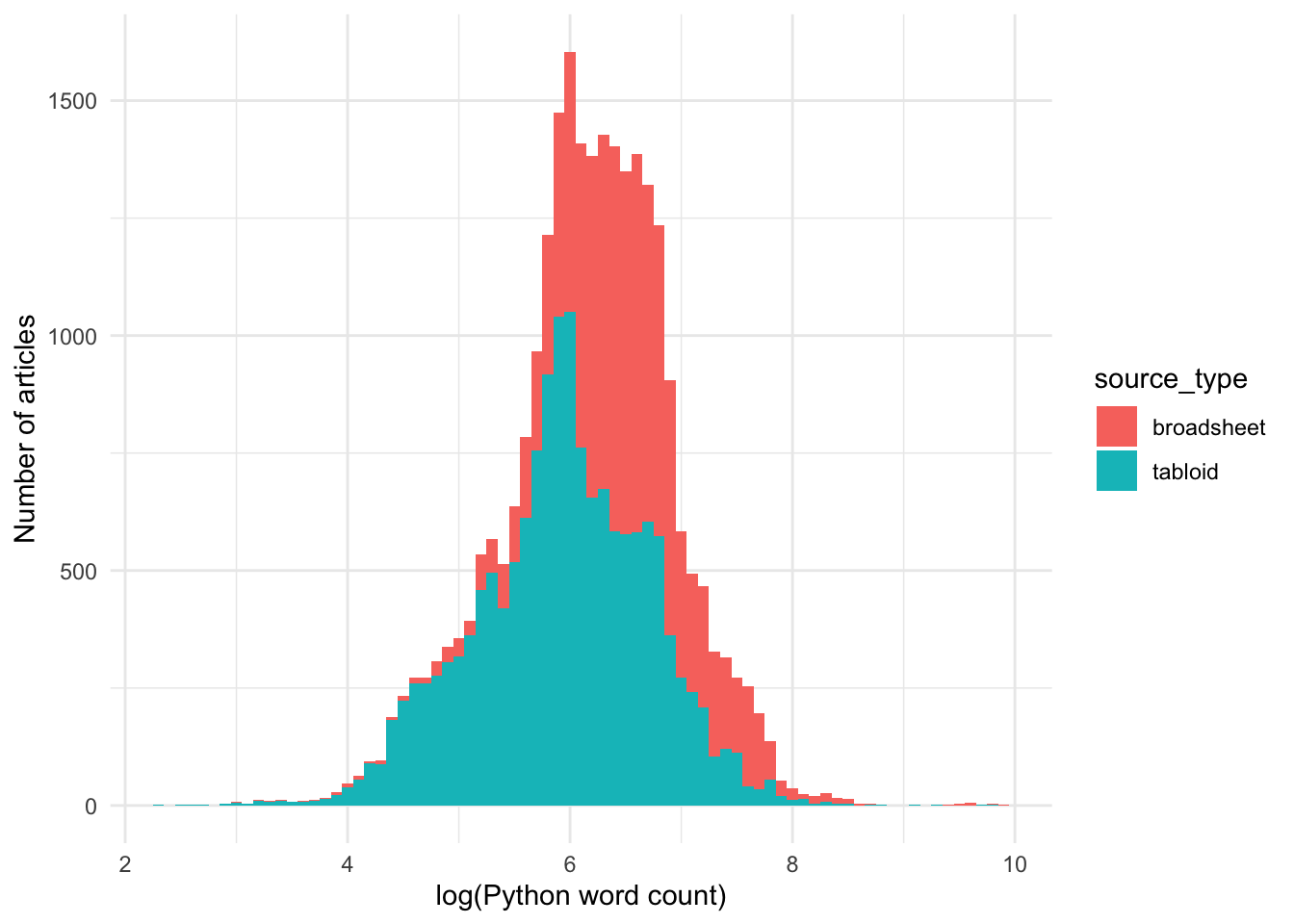
The log-transformed word count data is approximately normally distributed.

Let’s see if the difference in length of articles using the adjective lemma OBESE in tabloids and broadsheets is significant?

Code

wordcount_broadsheet <- metadata_full[metadata_full$source_type == "broadsheet","wordcount_total", drop = T]
wordcount_tabloid <- metadata_full[metadata_full$source_type == "tabloid","wordcount_total", drop = T]
report::report(t.test(wordcount_broadsheet,wordcount_tabloid))

The Welch Two Sample t-test testing the difference between wordcount_broadsheet and wordcount_tabloid (mean of x = 810.15, mean of y = 502.44) suggests that the effect is positive, statistically significant, and small (difference = 307.71, 95% CI [291.01, 324.42], t(16482.54) = 36.11, p < .001; Cohen’s d = 0.47, 95% CI [0.45, 0.50])

Yes, we can see that across the entire dataset, the word count of articles published in broadsheets are longer than that in tabloids.

This is supported by a non-parametric test as well:

Code

fp_test(wc1 = wordcount_broadsheet,
        wc2 = wordcount_tabloid,
        label1 = "broadsheet",
        label2 = "tabloid",
        dist = mydistribution)


    Approximative Two-Sample Fisher-Pitman Permutation Test
data:  wc by label (broadsheet, tabloid)
Z = 37.999, p-value < 1e-04
alternative hypothesis: true mu is not equal to 0

If we then test the difference between the frequency of the adjective lemma OBESE in tabloids and broadsheets, we can see that a higher frequency per 1000 words is detected for usage of the adjective lemma OBESE in tabloids than broadsheets.

Code

frequency_broadsheet <- obese_annotated_filtered[obese_annotated_filtered$source_type == "broadsheet","frequency", drop = T]
frequency_tabloid <- obese_annotated_filtered[obese_annotated_filtered$source_type == "tabloid","frequency", drop = T]
report::report(t.test(frequency_broadsheet, frequency_tabloid))

The Welch Two Sample t-test testing the difference between frequency_broadsheet and frequency_tabloid (mean of x = 3.16, mean of y = 5.59) suggests that the effect is negative, statistically significant, and small (difference = -2.43, 95% CI [-2.63, -2.23], t(10062.88) = -24.01, p < .001; Cohen’s d = -0.46, 95% CI [-0.50, -0.42])

So, yes, the frequency of use of the adjective lemma OBESE is higher in tabloids than in broadsheets.

This is supported by a non-parametric test as well:

Code

fp_test(wc1 = frequency_broadsheet,
        wc2 = frequency_tabloid,
        label1 = "broadsheet",
        label2 = "tabloid",
        dist = mydistribution)


    Approximative Two-Sample Fisher-Pitman Permutation Test
data:  wc by label (broadsheet, tabloid)
Z = -21.36, p-value < 1e-04
alternative hypothesis: true mu is not equal to 0

Let’s use bootstrapping to see if the raw frequencies of usage of OBESE are different?

Code

broadsheet_counts <- NULL
tabloid_counts <- NULL
for (i in 1:10000) {
  x <- mean(sample({obese_annotated_filtered %>% 
        filter(source_type == "broadsheet") %>%
        pull(no_hits_in_text)}, 1000, replace = FALSE))
  y <- mean(sample({obese_annotated_filtered %>% 
        filter(source_type == "tabloid") %>%
        pull(no_hits_in_text)}, 1000, replace = FALSE))
  broadsheet_counts <- c(broadsheet_counts, x)
  tabloid_counts <- c(tabloid_counts, y)
}
counts_comparison <- data.frame(
  mean_sample = c(broadsheet_counts, tabloid_counts),
  source_type = c(
    rep("broadsheet", length(broadsheet_counts)),
    rep("tabloid", length(tabloid_counts))))
counts_comparison %>%
  ggplot(aes(x = mean_sample, fill = source_type)) + 
  geom_histogram()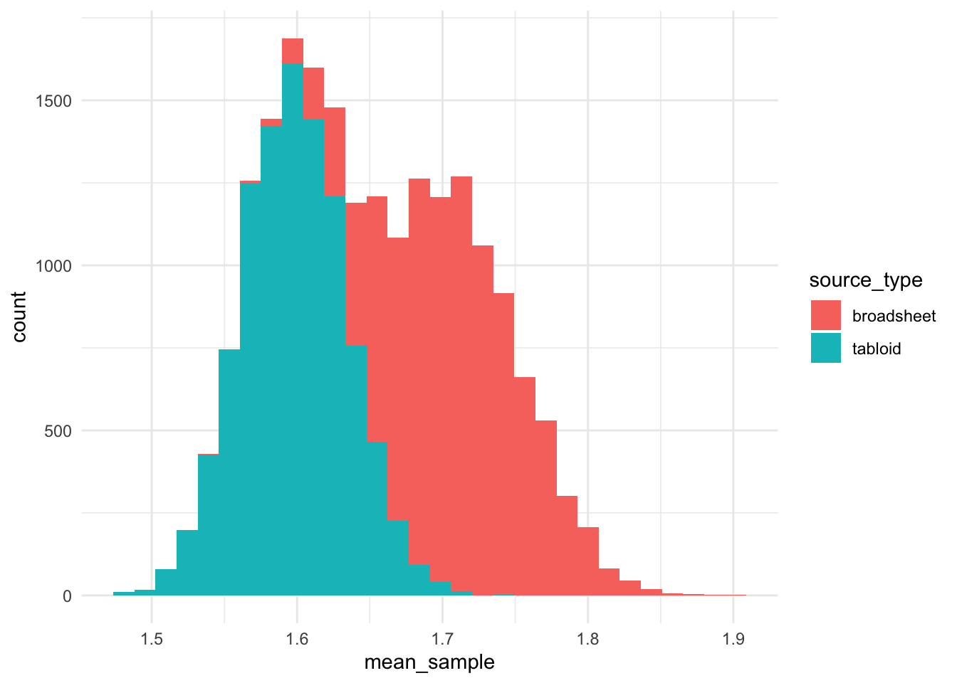

Figure 8: Histogram of sampling of counts per article of the raw frequency of use of OBESE in tabloids and broadsheets.

It is interesting that the distribution of usage of OBESE is ~1.6 uses per article in tabloid publications, while the distribution for broadsheets was bimodal.

Code

report::report(
  t.test(
    broadsheet_counts,
    tabloid_counts
  )
)

The Welch Two Sample t-test testing the difference between broadsheet_counts and tabloid_counts (mean of x = 1.71, mean of y = 1.60) suggests that the effect is positive, statistically significant, and large (difference = 0.11, 95% CI [0.11, 0.11], t(18734.64) = 186.07, p < .001; Cohen’s d = 2.63, 95% CI [2.89, 2.89])

This is supported by a non-parametric test as well:

Code

fp_test(wc1 = broadsheet_counts,
        wc2 = tabloid_counts,
        label1 = "broadsheet",
        label2 = "tabloid",
        dist = mydistribution)


    Approximative Two-Sample Fisher-Pitman Permutation Test
data:  wc by label (broadsheet, tabloid)
Z = 112.59, p-value < 1e-04
alternative hypothesis: true mu is not equal to 0

So the COUNT of instances of the adjective lemma OBESE is HIGHER in broadsheets than tabloids - the opposite result of when we consider the frequency. This is likely to be due to broadsheets having much longer articles than tabloids.

Let’s look at the trend over time:

Code

obese_annotated_filtered %>%
  ggplot(aes(x = as.factor(year), 
             y = log(frequency), 
             fill = year)) + 
  geom_jitter(alpha = 0.2) +
  geom_smooth(aes(group = source_type), col = "blue", method = "loess") +
  geom_hline(yintercept = 1, col = "red", lty = 3, size = 3) + 
  facet_wrap(~source_type) + 
  theme(axis.text.x = 
          element_text(angle = 90, vjust = 0.5, hjust=1),
        legend.position = "NA") + 
  labs(
    x = "Year",
    y = "log(frequency per 1000 words)"
  )

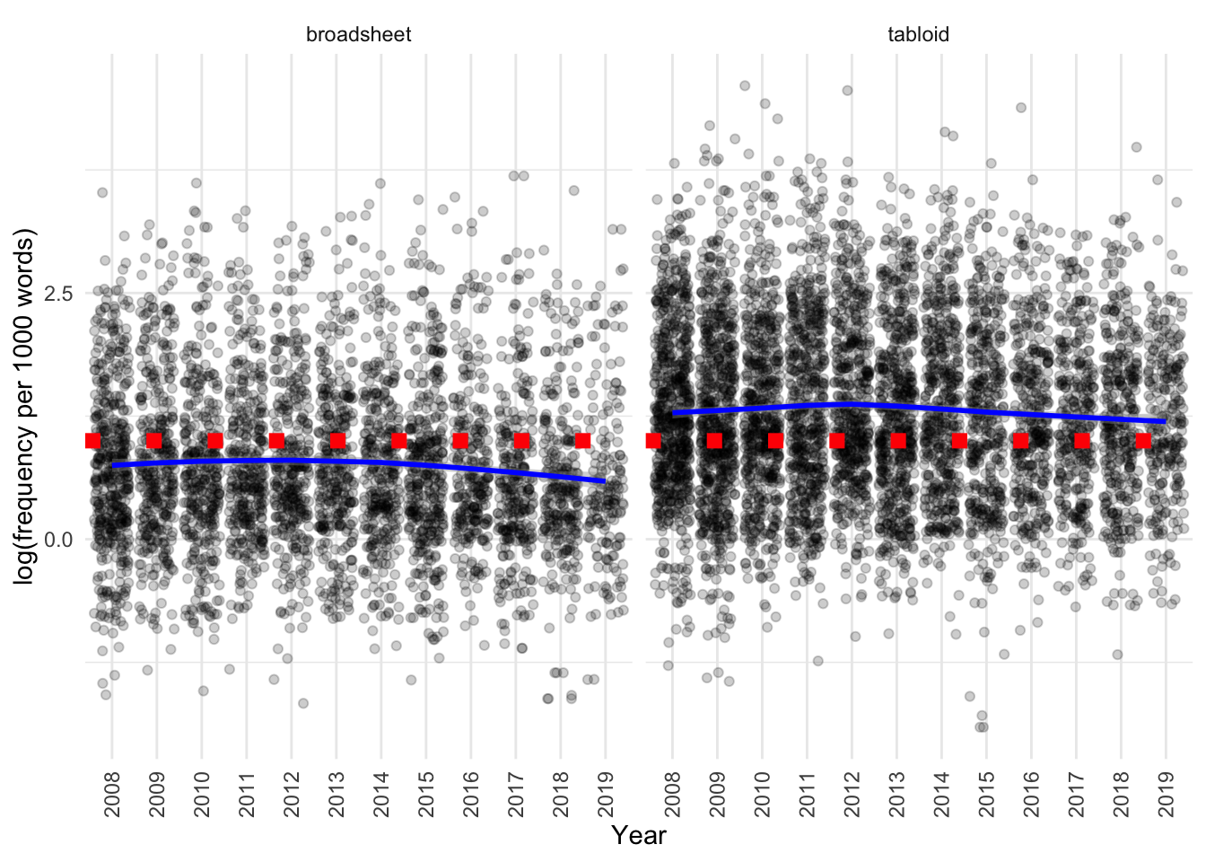
Figure 9: Raw and smoothed frequency of use of OBESE in the corpus in tabloids and broadsheets, by year and publication type.

We can see that there is a difference:

between tabloids and broadsheets, as characterised above
usage subtly decreases in both over time

Comparing observed to normalised to subcorpus size data

We can investigate the prevalence of the use of OBESE using goodness of fit tests, comparing the distribution in:

tabloids vs broadsheets
left and right leaning publications

We can do this by looking at:

the total number of instances in each subcorpus, normalised to the total number of words in each subcorpus
the number of articles that feature this language type, normalised to the total number of articles in each subcorpus

Tabloids vs broadsheets

The total number of uses of OBESE we observe is higher in tabloids and lower in broadsheets than we would expect based on the word count in these subcorpora (p < 0.001).

Code

chisq_instances_wc_normalised(obese_annotated_filtered, metadata_full, source_type) |> kable()

Table 3: Chi-Squared test for number of uses of OBESE in tabloids and broadsheets vs what would be expected given word count across all articles in the publication types.
variable	value
method	Chi-squared test for given probabilities
parameter	1
statistic	778.4111
p.value	2.666527e-171
broadsheet_observed	7071
broadsheet_expected	8878.82882136884
tabloid_observed	9773
tabloid_expected	7965.17117863116

The number of articles with use of OBESE we observe is not different between tabloids and broadsheets.

Code

chisq_articles_totalart_normalised(obese_annotated_filtered, metadata_full, source_type) |> kable()

Table 4: Chi-Squared test for number of articles that use OBESE in tabloids and broadsheets vs what would be expected given total number of articles in the publication types.
variable	value
method	Chi-squared test for given probabilities
parameter	1
statistic	1.012291
p.value	0.3143545
broadsheet_observed	4142
broadsheet_expected	4192.09050949815
tabloid_observed	6114
tabloid_expected	6063.90949050185

Left vs right-leaning publications

The total number of uses of OBESE we observe is higher in right and lower in left-leaning publications than we would expect based on the word count in these subcorpora (p < 0.001).

Code

chisq_instances_wc_normalised(obese_annotated_filtered, metadata_full, orientation) |> kable()

Table 5: Chi-Squared test for number of uses of OBESE in left and right leaning publications vs what would be expected given word count across all articles in the publication types.
variable	value
method	Chi-squared test for given probabilities
parameter	1
statistic	336.0413
p.value	4.645282e-75
left_observed	5938
left_expected	7113.11347665779
right_observed	10906
right_expected	9730.88652334221

The number of articles that use OBESE we observe is not different between left and right leaning publications.

Code

chisq_articles_totalart_normalised(obese_annotated_filtered, metadata_full, orientation) |> kable()

Table 6: Chi-Squared test for number of articles that use OBESE left and right leaning publications vs what would be expected given total number of articles in the publication types.
variable	value
method	Chi-squared test for given probabilities
parameter	1
statistic	0.03741104
p.value	0.8466306
left_observed	3433
left_expected	3423.7627183427
right_observed	6823
right_expected	6832.2372816573

Differences in usage by source

Is there a difference in the usage of OBESE by source?

Code

obese_annotated_filtered %>%
  ggplot(aes(x = reorder(source,frequency), 
             y = log(frequency), 
             fill = source_type)) + 
  geom_boxplot() +
  theme(axis.text.x = 
          element_text(angle = 90, vjust = 0.5, hjust=1),
        legend.position = "NA")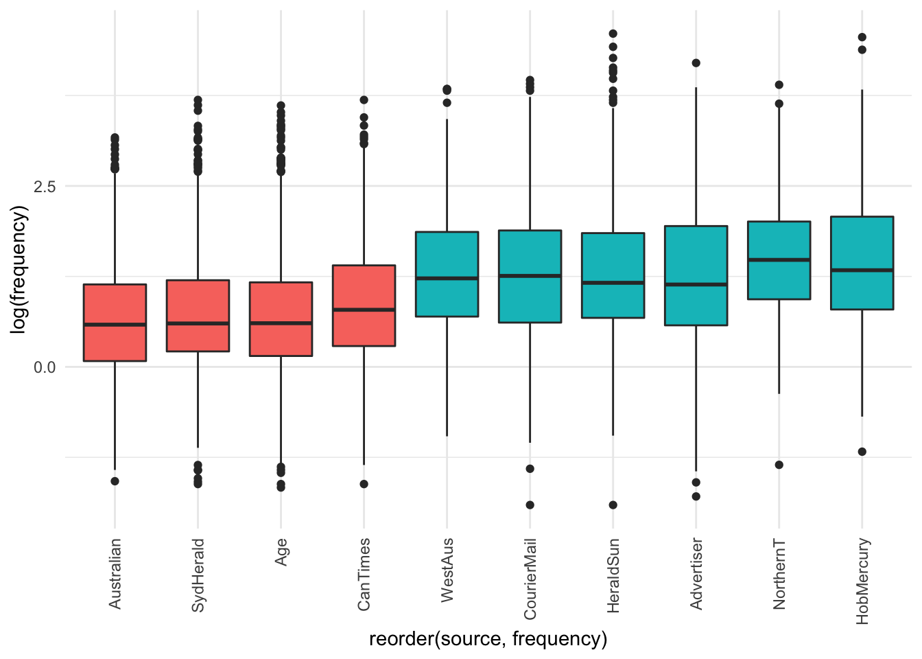

Figure 10: Box plot of usage of OBESE by source.

The visualisation suggests there is not - only the differences observed above for tabloids vs broadsheets.

What are the means and standard deviations of the frequency by source?

Code

obese_annotated_filtered %>% 
  group_by(source) %>%
  summarise(
    mean = mean(frequency),
    median = median(frequency),
    sd = sd(frequency),
    type = (source_type)
  ) %>%
  distinct() %>%
  arrange(mean) %>%
  kable()

Table 7: Mean, median and standard deviation of frequency of use of OBESE by source.
source	mean	median	sd	type
Australian	2.817048	1.792115	3.175300	broadsheet
SydHerald	3.072108	1.821494	3.657049	broadsheet
Age	3.154595	1.828154	4.060922	broadsheet
CanTimes	3.569830	2.200220	4.025436	broadsheet
WestAus	5.292246	3.397508	5.496833	tabloid
CourierMail	5.351845	3.514949	5.800857	tabloid
HeraldSun	5.493390	3.194888	6.965477	tabloid
Advertiser	5.565510	3.120132	6.236993	tabloid
NorthernT	6.251933	4.385965	6.097086	tabloid
HobMercury	6.464202	3.802281	8.143909	tabloid

It seems that within the different sources among broadsheets and tabloids there is not much difference among the frequency of use of the adjective lemma OBESE.

Differences in usage by year

Is there any year when OBESE is used more frequently than others?

Code

obese_annotated_filtered %>%
  ggplot(aes(x = reorder(year,frequency), 
             y = log(frequency), 
             fill = year)) + 
  geom_boxplot() +
  theme(axis.text.x = 
          element_text(angle = 90, vjust = 0.5, hjust=1),
        legend.position = "NA")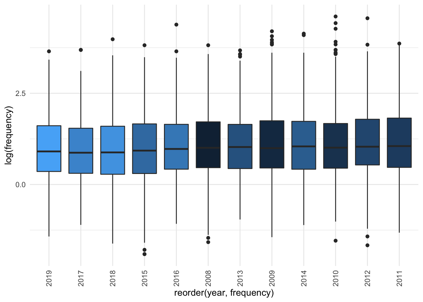

Figure 11: Use of OBESE by year, sorted by median use per year from least frequent to most frequent.

Based on the visualisation it seems not. If we separate out by source there also doesn’t seem to be much difference. If we use a jitter plot to visualise the data, then fit a smoothing line and compare with the line of “no change” (dashed red line), we can see that there really isn’t a very strong difference by source and year:

Code

obese_annotated_filtered %>%
  ggplot(aes(x = as.factor(year), 
             y = log(frequency), 
             fill = year)) + 
  geom_jitter(alpha = 0.2) +
  geom_smooth(aes(group = source), col = "blue", method = "loess") +
  geom_hline(yintercept = 1, col = "red", lty = 3, size = 3) + 
  facet_wrap(~source) + 
  theme(axis.text.x = 
          element_text(angle = 90, vjust = 0.5, hjust=1),
        legend.position = "NA") + 
  labs(
    x = "Year",
    y = "log(frequency per 1000 words)"
  )

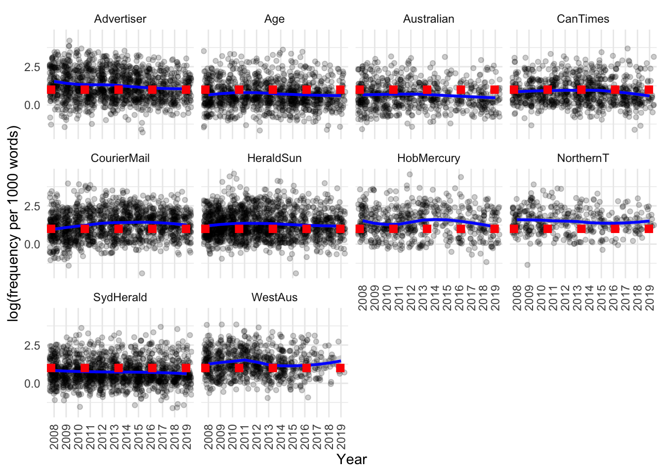
Figure 12: Use of OBESE by year and source, split by publication.

The distributions each year also look quite similar:

Code

obese_annotated_filtered %>%
  ggplot(aes(x = reorder(year,frequency), 
             y = log(frequency), 
             fill = year)) + 
  geom_violin() +
  theme(axis.text.x = 
          element_text(angle = 90, vjust = 0.5, hjust=1),
        legend.position = "NA") +
  labs(x = "Year")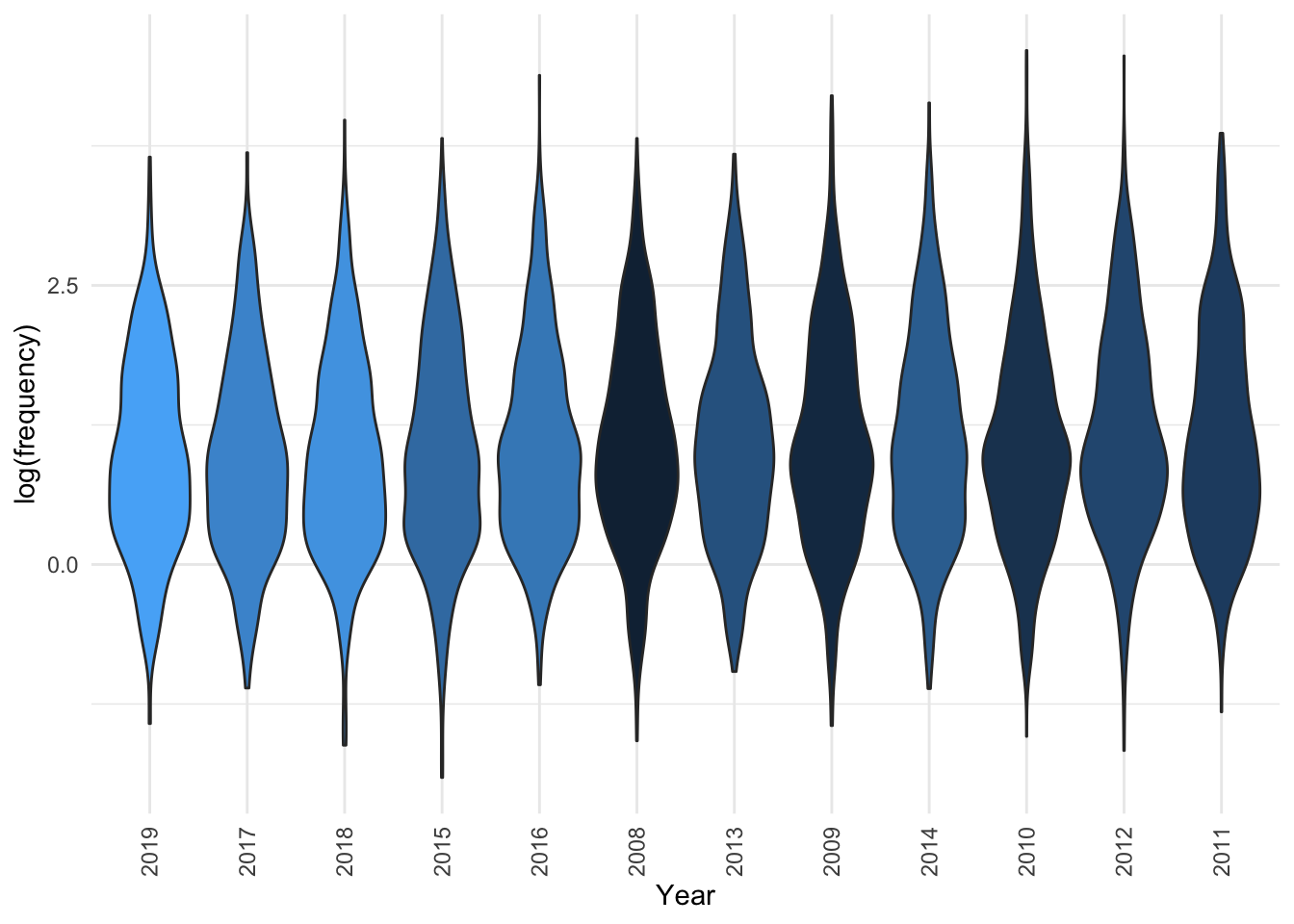

Figure 13: Violin plot of the distributions of use of OBESE by year.

Code

obese_annotated_filtered %>% 
  group_by(year) %>%
  summarise(
    mean = mean(frequency),
    median = median(frequency),
    sd = sd(frequency),
    year = (year)
  ) %>%
  distinct() %>%
  arrange(mean) %>%
  kable()

Table 8: Descriptive statistics of the use of OBESE by year across the dataset.
year	mean	median	sd
2019	3.817842	2.475248	3.971667
2017	3.866365	2.389490	4.300584
2018	3.966531	2.409639	4.616181
2015	4.335848	2.531646	4.950555
2016	4.471581	2.649011	5.673864
2008	4.512463	2.732240	4.882211
2013	4.581882	2.793296	5.057143
2009	4.801149	2.706365	6.176861
2014	4.926691	2.840909	6.018102
2010	4.938758	2.743489	7.376403
2012	5.065254	2.816924	6.234889
2011	5.128600	2.865330	6.218089

Differences in usage by source type, source and year

We can also try to simultaneously model differences by source type, source and year.

As expected, a model that includes the source type (tabloid vs broadsheet) gives a better fit than one that does not:

Code

obese_annotated_filtered$scaled_year <- scale(
  obese_annotated_filtered$year, scale = F)
library(lme4)
# base model
m_0_base <- lm(log(frequency) ~ 1, 
                data = obese_annotated_filtered)
# with source type
m_0_sourcetype <- lm(log(frequency) ~ source_type,  
                data = obese_annotated_filtered)
# with year
m_0_year <- lm(log(frequency) ~ scaled_year,  
                data = obese_annotated_filtered)
# with source 
m_0_source <- lm(log(frequency) ~ source,  
                data = obese_annotated_filtered)
# with source and year
# with source 
m_0_sourceyear <- lm(log(frequency) ~ source + scaled_year,  
                data = obese_annotated_filtered)
# compare
rbind({broom::glance(m_0_base) %>% 
    dplyr::select(-df.residual,- deviance, -nobs) %>%
    mutate(model = "1")},
    {broom::glance(m_0_sourcetype)%>% 
          dplyr::select(-df.residual,- deviance, -nobs) %>%
        mutate(model = "source_type")},
    {broom::glance(m_0_year) %>% 
    dplyr::select(-df.residual,- deviance, -nobs) %>%
    mutate(model = "scaled_year")},
    {broom::glance(m_0_source) %>% 
    dplyr::select(-df.residual,- deviance, -nobs) %>%
    mutate(model = "source")},
    {broom::glance(m_0_sourceyear) %>% 
    dplyr::select(-df.residual,- deviance, -nobs) %>%
    mutate(model = "sourceyear")}
) %>% 
  dplyr::select(model, everything()) %>%
  arrange(AIC) %>%
  kable()

Table 9: Comparison of model summary statistics for simple linear models that incorporate source, scaled year and/or source type.
model	r.squared	adj.r.squared	sigma	statistic	p.value	df	logLik	AIC	BIC
sourceyear	0.0965926	0.0957108	0.8690119	109.53982	0e+00	10	-13107.20	26238.41	26325.24
source	0.0952110	0.0944163	0.8696337	119.79863	0e+00	9	-13115.04	26252.08	26331.67
source_type	0.0891430	0.0890541	0.8722045	1003.52945	0e+00	1	-13149.32	26304.63	26326.34
scaled_year	0.0026045	0.0025072	0.9126977	26.77577	2e-07	1	-13614.74	27235.48	27257.19
1	0.0000000	0.0000000	0.9138440	NA	NA	NA	-13628.12	27260.23	27274.70

We can see that the model incorporating source and year provides the best fit for the data, explaining somewhat more variability than that which includes only source type.

Code

anova(m_0_sourcetype, m_0_sourceyear)

Analysis of Variance Table
Model 1: log(frequency) ~ source_type
Model 2: log(frequency) ~ source + scaled_year
  Res.Df    RSS Df Sum of Sq      F    Pr(>F)    
1  10254 7800.6                                  
2  10245 7736.8  9    63.799 9.3868 2.396e-14 ***
---
Signif. codes:  0 '***' 0.001 '**' 0.01 '*' 0.05 '.' 0.1 ' ' 1

Next, let’s compare if having a distinct intercept for each source improves the fit of the model.

Code

m_1_source <- lmer(log(frequency) ~  1 + (1|source), 
                data = obese_annotated_filtered, REML = T)
m_1_sourceyear <- lmer(log(frequency) ~  scaled_year + (1|source), 
                data = obese_annotated_filtered, REML = T)
m_1_sourceyear2 <- lmer(log(frequency) ~  scaled_year + (scaled_year|source), 
                data = obese_annotated_filtered, REML = T)
m_1_sourceyeartype <- lmer(log(frequency) ~  scaled_year + source_type + (1|source), 
                data = obese_annotated_filtered, REML = T)
m_1_sourceyeartype2 <- lmer(log(frequency) ~  scaled_year + source_type + (scaled_year|source), 
                data = obese_annotated_filtered, REML = T)
rbind(
    {broom::glance(m_0_sourceyear)%>% 
          dplyr::select(AIC, BIC, logLik) %>%
        mutate(model = "scaled_year + source")},
    {broom.mixed::glance(m_1_source) %>% 
    dplyr::select(AIC, BIC, logLik) %>%
    mutate(model = "1 + (1/source)")},
    {broom.mixed::glance(m_1_sourceyear)%>% 
          dplyr::select(AIC, BIC, logLik) %>%
        mutate(model = "scaled_year + 1/source")},
    {broom.mixed::glance(m_1_sourceyeartype)%>% 
          dplyr::select(AIC, BIC, logLik) %>%
        mutate(model = "scaled_year + source_type + 1/source")},
    {broom.mixed::glance(m_1_sourceyear2)%>% 
          dplyr::select(AIC, BIC, logLik) %>%
        mutate(model = "scaled_year + scaled_year/source")},
    {broom.mixed::glance(m_1_sourceyeartype2)%>% 
          dplyr::select(AIC, BIC, logLik) %>%
        mutate(model = "scaled_year + source_type + scaled_year/source")}
) %>%
  arrange(AIC) %>%
  kable()

Table 10: Comparison of model summary statistics for linear mixed effects models that incorporate source, scaled year and/or source type.
AIC	BIC	logLik	model
26238.41	26325.24	-13107.20	scaled_year + source
26239.73	26290.38	-13112.86	scaled_year + source_type + scaled_year/source
26256.38	26299.79	-13122.19	scaled_year + scaled_year/source
26275.94	26312.12	-13132.97	scaled_year + source_type + 1/source
26292.53	26321.47	-13142.26	scaled_year + 1/source
26296.20	26317.91	-13145.10	1 + (1/source)

Including a distinct intercept for each source did not drastically improve the fit of the model (AIC increases, logLik decreases; BIC does decrease slightly, so based on this criteria it may be a slightly better fit).

Let’s plot the residuals for the fixed effects model:

Code

source(here::here("400_analysis","model_diagnostics.R"))
df_model_resid <- get_model_resid_df(m_0_sourceyear)
diagnostic_lm_plot(df_model_resid)

Figure 14: Plot of model residuals for the fixed effects model log(frequency) ~ source + scaled_year.

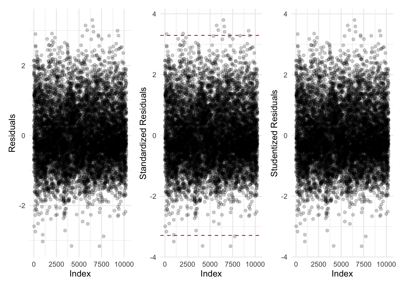
Proportion of data points with:

abs(standardized residuals) > 3.29: 0.13%
abs(standardized residuals) > 2.58: 1.02%
abs(standardized residuals) > 1.96: 4.93%

All of these indicate the model is performing reasonably well on the data.

Let’s summarise the model (note that the intercept corresponds to the “first” source, i.e. the Advertiser):

Code

sjPlot::tab_model(m_0_sourceyear)

Table 11: Coefficients and confidence intervals for the fixed effects model log(frequency) ~ source + scaled_year.
	log(frequency)
Predictors	Estimates	CI	p
(Intercept)	1.27	1.22 – 1.31	<0.001
source [Age]	-0.55	-0.62 – -0.48	<0.001
source [Australian]	-0.63	-0.71 – -0.55	<0.001
source [CanTimes]	-0.37	-0.44 – -0.30	<0.001
source [CourierMail]	0.01	-0.06 – 0.07	0.816
source [HeraldSun]	0.02	-0.05 – 0.08	0.628
source [HobMercury]	0.14	0.06 – 0.23	0.001
source [NorthernT]	0.23	0.13 – 0.33	<0.001
source [SydHerald]	-0.52	-0.59 – -0.46	<0.001
source [WestAus]	0.02	-0.05 – 0.10	0.552
scaled year	-0.01	-0.02 – -0.01	<0.001
Observations	10256
R² / R² adjusted	0.097 / 0.096

In summary, the fixed effects model which included source and year provided a good fit. Let’s summarise this model:

Code

report::report(m_0_sourceyear)

We fitted a linear model (estimated using OLS) to predict frequency with source and scaled_year (formula: log(frequency) ~ source + scaled_year). The model explains a statistically significant and weak proportion of variance (R2 = 0.10, F(10, 10245) = 109.54, p < .001, adj. R2 = 0.10). The model’s intercept, corresponding to source = Advertiser and scaled_year = 0, is at 1.27 (95% CI [1.22, 1.31], t(10245) = 54.39, p < .001). Within this model:

The effect of source [Age] is statistically significant and negative (beta = -0.55, 95% CI [-0.62, -0.48], t(10245) = -15.82, p < .001; Std. beta = -0.21, 95% CI [-0.23, -0.18])
The effect of source [Australian] is statistically significant and negative (beta = -0.63, 95% CI [-0.71, -0.55], t(10245) = -15.68, p < .001; Std. beta = -0.23, 95% CI [-0.27, -0.20])
The effect of source [CanTimes] is statistically significant and negative (beta = -0.37, 95% CI [-0.44, -0.30], t(10245) = -9.90, p < .001; Std. beta = -0.16, 95% CI [-0.19, -0.13])
The effect of source [CourierMail] is statistically non-significant and positive (beta = 7.70e-03, 95% CI [-0.06, 0.07], t(10245) = 0.23, p = 0.816; Std. beta = -6.00e-03, 95% CI [-0.03, 0.02])
The effect of source [HeraldSun] is statistically non-significant and positive (beta = 0.02, 95% CI [-0.05, 0.08], t(10245) = 0.48, p = 0.628; Std. beta = -8.24e-03, 95% CI [-0.03, 0.02])
The effect of source [HobMercury] is statistically significant and positive (beta = 0.14, 95% CI [0.06, 0.23], t(10245) = 3.31, p < .001; Std. beta = 0.06, 95% CI [0.02, 0.09])
The effect of source [NorthernT] is statistically significant and positive (beta = 0.23, 95% CI [0.13, 0.33], t(10245) = 4.44, p < .001; Std. beta = 0.07, 95% CI [0.03, 0.11])
The effect of source [SydHerald] is statistically significant and negative (beta = -0.52, 95% CI [-0.59, -0.46], t(10245) = -16.02, p < .001; Std. beta = -0.21, 95% CI [-0.23, -0.18])
The effect of source [WestAus] is statistically non-significant and positive (beta = 0.02, 95% CI [-0.05, 0.10], t(10245) = 0.59, p = 0.552; Std. beta = -0.01, 95% CI [-0.04, 0.02])
The effect of scaled year is statistically significant and negative (beta = -0.01, 95% CI [-0.02, -5.16e-03], t(10245) = -3.96, p < .001; Std. beta = -0.02, 95% CI [-0.02, -8.05e-03])

Standardized parameters were obtained by fitting the model on a standardized version of the dataset. 95% Confidence Intervals (CIs) and p-values were computed using the Wald approximation.

To summarise, a model was fit by source and year, which explained a small amount of variance in the data. It showed that the Age, Australian, Canberra Times and Sydney Morning Herald had a lower frequency of use of the adjective lemma OBESE relative to the Advertiser, while in the Hobart Mercury, Northern Territorian the adjective lemma OBESE was used somewhat more frequently than in the Advertiser. Use of the adjective lemma OBESE decreased with time in the corpus.

If we look at the mixed effects model scaled_year + source_type + scaled_year/source, which had the lowest BIC, we can see that the observation of higher frequency of counts in tabloids is reproduced, while the signal from the decrease by year is not detected:

Code

sjPlot::tab_model(m_1_sourceyeartype2)

Table 12: Coefficients and confidence intervals for the mixed effects model scaled_year + source_type + scaled_year/source.
	log(frequency)
Predictors	Estimates	CI	p
(Intercept)	0.75	0.65 – 0.84	<0.001
scaled year	-0.01	-0.02 – 0.00	0.054
source type [tabloid]	0.58	0.46 – 0.70	<0.001
Random Effects
σ²	0.75
τ₀₀_source	0.01
τ₁₁_{source.scaled_year}	0.00
ρ₀₁_source	-0.18
ICC	0.02
N _source	10
Observations	10256
Marginal R² / Conditional R²	0.100 / 0.114

The intercepts and slopes for scaled year for each of the sources were:

Code

coef(m_1_sourceyeartype2)$source %>% 
  arrange(`(Intercept)`) %>% 
  kable()

Table 13: Intercepts and coefficients for the mixed effects model scaled_year + source_type + scaled_year/source.
	(Intercept)	scaled_year	source_typetabloid
Australian	0.6482964	-0.0153703	0.5831533
CourierMail	0.6838377	0.0273333	0.5831533
Advertiser	0.6941022	-0.0378463	0.5831533
HeraldSun	0.7009579	-0.0077894	0.5831533
WestAus	0.7057935	-0.0152603	0.5831533
Age	0.7172206	-0.0107049	0.5831533
SydHerald	0.7434942	-0.0139594	0.5831533
HobMercury	0.8135840	-0.0111710	0.5831533
NorthernT	0.8725238	-0.0212058	0.5831533
CanTimes	0.8825098	-0.0163459	0.5831533

Differences in usage by topic

Code

metadata_full %>%
  group_by(source_type) %>%
  count(topic_label) %>%
  pivot_wider(names_from = source_type, values_from = n) %>%
  mutate(
    total_topic = broadsheet + tabloid,
    prop_broadsheet = round(100*broadsheet/total_topic, 2)
  ) %>% 
  arrange(prop_broadsheet) %>%
  kable()

Table 14: Number of articles published on various topics in tabloids and broadsheets, with topics predicted using topic modelling analysis.
topic_label	broadsheet	tabloid	total_topic	prop_broadsheet
ChildrenParents	364	1335	1699	21.42
NutritionStudy	642	1797	2439	26.32
WomenPregnancy	159	385	544	29.23
FitnessExercise	464	1093	1557	29.80
BiomedResearch	1013	2077	3090	32.78
MedicalHealth	297	524	821	36.18
Food	539	800	1339	40.25
FastFood&Drinks	1044	1441	2485	42.01
Transport&Commuting	427	559	986	43.31
WomenGirls	625	744	1369	45.65
Awards	28	33	61	45.90
PublicHealthReport	1243	1338	2581	48.16
Students&Teachers	536	572	1108	48.38
Microbiome	32	33	65	49.23
SportsDoping	260	253	513	50.68
Politics	1478	1249	2727	54.20
MusicMovies	1543	1236	2779	55.52

We can see that articles labelled with the topics “ChildrenParents”, “NutritionStudy”, “WomenPregnancy” and “FitnessExercise” are approximately 3x more frequently reported on in tabloids than broadsheets, in contrast to topics like “Politics” and “SportsDoping” which are approximately evenly represented between the two media types.

Code

obese_annotated_filtered %>%
  ggplot(aes(x = as.factor(
    reorder(topic_label,frequency)), 
             y = log(frequency), 
             fill = topic_label)) + 
  geom_boxplot() +
  theme(axis.text.x = 
          element_text(angle = 90, vjust = 0.5, hjust=1),
        legend.position = "NA") +
  labs(x = "Topic label",
       y = "log(frequency per 1000 words)")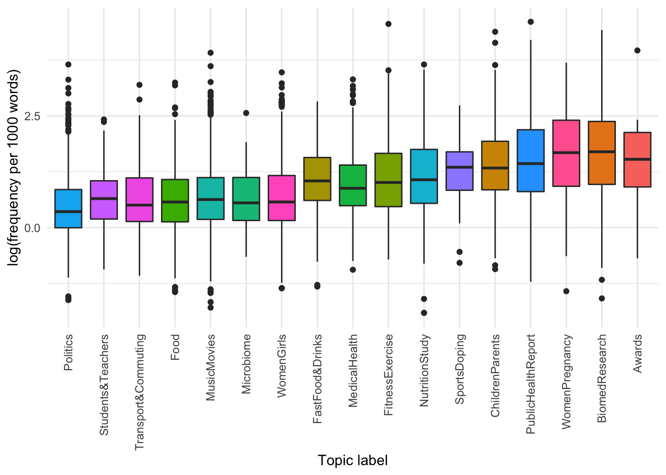

Figure 15: Frequency of use of OBESE per 1000 words in articles annotated with specific topic lables.

It seems there are some topics that use OBESE more than others.

We use a simple linear model with post-hoc comparisons and Bonferroni multiple testing correction:

Code

obese_by_topic <- lm(
  frequency ~ as.factor(topic_label), 
  data = obese_annotated_filtered)
library(emmeans)
obese_by_topic_comp <- emmeans(obese_by_topic, pairwise ~ as.factor(topic_label), adjust = "bonferroni")
obese_by_topic_comp$contrasts %>%
    summary(infer = TRUE) %>%
  filter(p.value < 0.01) %>% 
  select(-df) |>
  kable()

Table 15: Differences in use of OBESE in articles annoated with specific topics, with topics compared pairwise with each other.
contrast	estimate	SE	lower.CL	upper.CL	t.ratio	p.value
Awards - Food	5.942155	1.4853012	0.6493259	11.2349838	4.000640	0.0086518
Awards - Politics	6.288435	1.4729512	1.0396145	11.5372546	4.269276	0.0026911
Awards - Students&Teachers	6.172930	1.4968448	0.8389660	11.5068943	4.123961	0.0051048
Awards - Transport&Commuting	5.942849	1.4971190	0.6079082	11.2777906	3.969524	0.0098612
BiomedResearch - ChildrenParents	2.635277	0.2323342	1.8073605	3.4631932	11.342613	0.0000000
BiomedResearch - FastFood&Drinks	4.493757	0.2333711	3.6621454	5.3253683	19.255838	0.0000000
BiomedResearch - FitnessExercise	3.872260	0.2219288	3.0814229	4.6630966	17.448211	0.0000000
BiomedResearch - Food	5.623753	0.2991564	4.5577179	6.6897886	18.798706	0.0000000
BiomedResearch - MedicalHealth	4.461614	0.3299740	3.2857608	5.6374669	13.521107	0.0000000
BiomedResearch - Microbiome	5.446934	1.1570708	1.3237445	9.5701229	4.707520	0.0003455
BiomedResearch - MusicMovies	5.496256	0.1920506	4.8118893	6.1806227	28.618798	0.0000000
BiomedResearch - NutritionStudy	3.717134	0.2237552	2.9197880	4.5144790	16.612498	0.0000000
BiomedResearch - Politics	5.970033	0.2301306	5.1499692	6.7900968	25.941938	0.0000000
BiomedResearch - PublicHealthReport	1.510443	0.2134401	0.7498552	2.2710307	7.076659	0.0000000
BiomedResearch - Students&Teachers	5.854529	0.3520215	4.6001098	7.1089473	16.631166	0.0000000
BiomedResearch - Transport&Commuting	5.624448	0.3531856	4.3658810	6.8830145	15.924909	0.0000000
BiomedResearch - WomenGirls	5.197677	0.2446344	4.3259286	6.0694243	21.246710	0.0000000
ChildrenParents - FastFood&Drinks	1.858480	0.2705723	0.8943035	2.8226567	6.868701	0.0000000
ChildrenParents - FitnessExercise	1.236983	0.2607674	0.3077457	2.1662201	4.743626	0.0002894
ChildrenParents - Food	2.988476	0.3290012	1.8160898	4.1608630	9.083481	0.0000000
ChildrenParents - MedicalHealth	1.826337	0.3572536	0.5532740	3.0994000	5.112159	0.0000441
ChildrenParents - MusicMovies	2.860979	0.2358616	2.0204932	3.7014651	12.129909	0.0000000
ChildrenParents - NutritionStudy	1.081857	0.2623236	0.1470739	2.0166394	4.124130	0.0051011
ChildrenParents - Politics	3.334756	0.2677823	2.3805216	4.2889907	12.453238	0.0000000
ChildrenParents - PublicHealthReport	-1.124834	0.2535822	-2.0284669	-0.2212008	-4.435776	0.0012607
ChildrenParents - Students&Teachers	3.219252	0.3777121	1.8732854	4.5652181	8.523031	0.0000000
ChildrenParents - Transport&Commuting	2.989171	0.3787972	1.6393379	4.3390039	7.891218	0.0000000
ChildrenParents - WomenGirls	2.562400	0.2803449	1.5633986	3.5614007	9.140169	0.0000000
ChildrenParents - WomenPregnancy	-2.125124	0.3656700	-3.4281787	-0.8220691	-5.811589	0.0000009
FastFood&Drinks - MusicMovies	1.002499	0.2368831	0.1583730	1.8466252	4.232042	0.0031769
FastFood&Drinks - Politics	1.476276	0.2686824	0.5188338	2.4337183	5.494502	0.0000055
FastFood&Drinks - PublicHealthReport	-2.983314	0.2545326	-3.8903337	-2.0762942	-11.720753	0.0000000
FastFood&Drinks - WomenPregnancy	-3.983604	0.3663297	-5.2890096	-2.6781982	-10.874367	0.0000000
FitnessExercise - Food	1.751494	0.3217375	0.6049911	2.8979959	5.443859	0.0000073
FitnessExercise - MusicMovies	1.623996	0.2256189	0.8200098	2.4279827	7.197963	0.0000000
FitnessExercise - Politics	2.097773	0.2588060	1.1755254	3.0200210	8.105582	0.0000000
FitnessExercise - PublicHealthReport	-2.361817	0.2440843	-3.2316042	-1.4920294	-9.676235	0.0000000
FitnessExercise - Students&Teachers	1.982269	0.3714022	0.6587875	3.3057501	5.337256	0.0000131
FitnessExercise - Transport&Commuting	1.752188	0.3725057	0.4247745	3.0796015	4.703789	0.0003519
FitnessExercise - WomenGirls	1.325417	0.2717838	0.3569227	2.2939107	4.876731	0.0001489
FitnessExercise - WomenPregnancy	-3.362107	0.3591487	-4.6419229	-2.0822907	-9.361323	0.0000000
Food - NutritionStudy	-1.906620	0.3230001	-3.0576213	-0.7556181	-5.902846	0.0000005
Food - PublicHealthReport	-4.113310	0.3159419	-5.2391605	-2.9874601	-13.019197	0.0000000
Food - WomenPregnancy	-5.113600	0.4113757	-6.5795258	-3.6476747	-12.430488	0.0000000
MedicalHealth - Politics	1.508419	0.3558244	0.2404489	2.7763894	4.239223	0.0030772
MedicalHealth - PublicHealthReport	-2.951171	0.3452646	-4.1815114	-1.7208304	-8.547564	0.0000000
MedicalHealth - WomenPregnancy	-3.951461	0.4343020	-5.4990839	-2.4038379	-9.098417	0.0000000
Microbiome - WomenPregnancy	-4.936781	1.1910282	-9.1809762	-0.6925853	-4.144974	0.0046592
MusicMovies - NutritionStudy	-1.779122	0.2274157	-2.5895120	-0.9687330	-7.823217	0.0000000
MusicMovies - PublicHealthReport	-3.985813	0.2172744	-4.7600643	-3.2115618	-18.344603	0.0000000
MusicMovies - WomenPregnancy	-4.986103	0.3414950	-6.2030107	-3.7691954	-14.600810	0.0000000
NutritionStudy - Politics	2.252899	0.2603739	1.3250644	3.1807345	8.652555	0.0000000
NutritionStudy - PublicHealthReport	-2.206691	0.2457462	-3.0824000	-1.3309811	-8.979553	0.0000000
NutritionStudy - Students&Teachers	2.137395	0.3724965	0.8100143	3.4647759	5.738027	0.0000013
NutritionStudy - Transport&Commuting	1.907314	0.3735967	0.5760128	3.2386157	5.105275	0.0000457
NutritionStudy - WomenGirls	1.480543	0.2732773	0.5067270	2.4543590	5.417731	0.0000084
NutritionStudy - WomenPregnancy	-3.206980	0.3602802	-4.4908287	-1.9231323	-8.901352	0.0000000
Politics - PublicHealthReport	-4.459590	0.2515648	-5.3560340	-3.5631460	-17.727402	0.0000000
Politics - WomenPregnancy	-5.459880	0.3642739	-6.7579598	-4.1618003	-14.988392	0.0000000
PublicHealthReport - Students&Teachers	4.344086	0.3663931	3.0384541	5.6497171	11.856351	0.0000000
PublicHealthReport - Transport&Commuting	4.114005	0.3675116	2.8043875	5.4236221	11.194217	0.0000000
PublicHealthReport - WomenGirls	3.687234	0.2648976	2.7432783	4.6311888	13.919465	0.0000000
Students&Teachers - WomenPregnancy	-5.344376	0.4512810	-6.9525027	-3.7362485	-11.842678	0.0000000
Transport&Commuting - WomenPregnancy	-5.114295	0.4521896	-6.7256596	-3.5029300	-11.310067	0.0000000
WomenGirls - WomenPregnancy	-4.687524	0.3736059	-6.0188577	-3.3561893	-12.546705	0.0000000

We can see that there are differences in the frequency of use of the adjective lemma OBESE by topic, with articles annotated as “Awards” and “Bio-medical Research” using more instances per 1000 words than articles discussing politics, schooling, transport and commuting.