In the below document, we show that we should use the Python-generated total word count for calculating normalised frequencies (or the counts provided in the metadata, as the two are nearly identical and well correlated across all text lengths.
In this file, we start by loading and exploring the data for the Australian Obesity Corpus.
Code
library(here)library(janitor)library(readr)library(dplyr)library(ggplot2)library(tidyr)library(knitr)theme_set(theme_minimal())read_cqpweb<-function(filename){read.csv(here("100_data_raw", filename),
skip =3, sep ="\t")%>%janitor::clean_names()}clean_fatneglabel<-function(dirname){purrr::map_dfr(list.files(here("100_data_raw", dirname)),
~{read.csv(here(paste0("100_data_raw/", dirname), .x),
skip =3, sep ="\t")%>%janitor::clean_names()})}condition_first<-read_cqpweb("aoc_all_condition_first.txt")person_first<-read_cqpweb("aoc_all_person_first.txt")adj_obese<-read_cqpweb("aoc_all_obese_tagadjlemma.txt")adj_overweight<-read_cqpweb("aoc_all_overweight_tagadjlemma.txt")fat_labelled<-clean_fatneglabel("fat_neg_label_yes_textFreqs")metadata<-read_csv(here("100_data_raw", "corpus_cqpweb_metadata.csv"))additional_source_metadata<-read_csv(here("100_data_raw", "addition_source_metadata.csv"))metadata_full<-inner_join(metadata, additional_source_metadata)condition_first_annotated<-inner_join(condition_first, metadata_full, by =c("text"="article_id"))person_first_annotated<-inner_join(person_first, metadata_full, by =c("text"="article_id"))fat_annotated<-inner_join(fat_labelled, metadata_full, by =c("text"="article_id"))write_csv(fat_annotated, file =here::here("200_data_clean", "fat_annotated.csv"))
Check that all text in the CQP web export file are found in the article_id of the metadata file, to ensure that there was no corruption of article_ids when we imported and exported from CQPWeb.
Table 2: Number of articles by source and month of publication.
source
01
02
03
04
05
06
07
08
09
10
11
12
Total
Advertiser
19
14
16
23
21
16
10
14
12
11
9
9
174
Age
9
6
4
0
12
12
9
10
13
15
16
14
120
Australian
8
11
11
6
11
7
10
14
3
8
9
6
104
BrisTimes
4
2
2
6
3
5
6
3
6
5
3
3
48
CanTimes
11
6
10
10
9
0
5
5
5
6
4
1
72
CourierMail
15
24
17
24
0
16
18
18
17
17
8
19
193
HeraldSun
16
23
10
20
15
17
14
16
12
14
6
13
176
HobMercury
7
17
15
10
1
8
7
8
4
3
9
5
94
NorthernT
3
7
3
2
3
2
5
3
1
6
1
4
40
SydHerald
15
14
18
14
22
19
17
17
19
22
21
16
214
Telegraph
13
20
9
23
10
18
13
12
7
10
8
6
149
WestAus
1
0
3
1
1
2
0
2
2
3
0
2
17
Total
121
144
118
139
108
122
114
122
101
120
94
98
1401
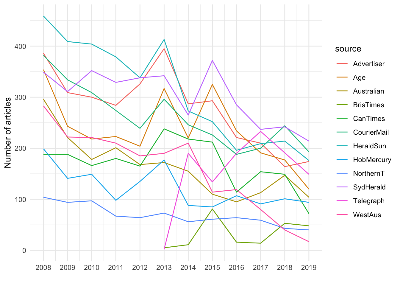
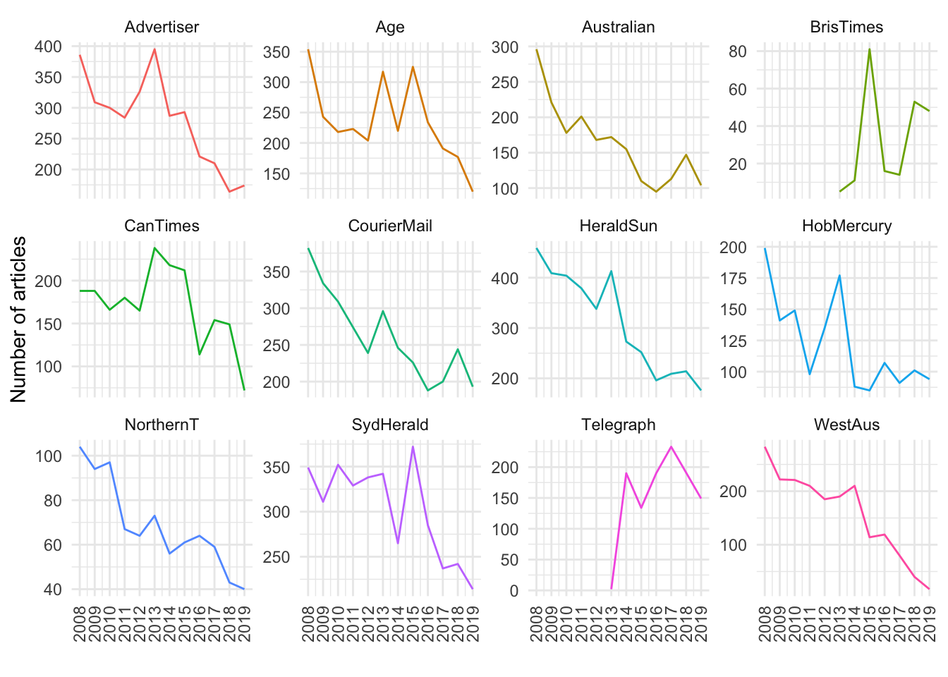
We can see that we do have data for each month from 2019, although there are many fewer articles that year from the Western Australian and to a lesser extent the Canberra Times.
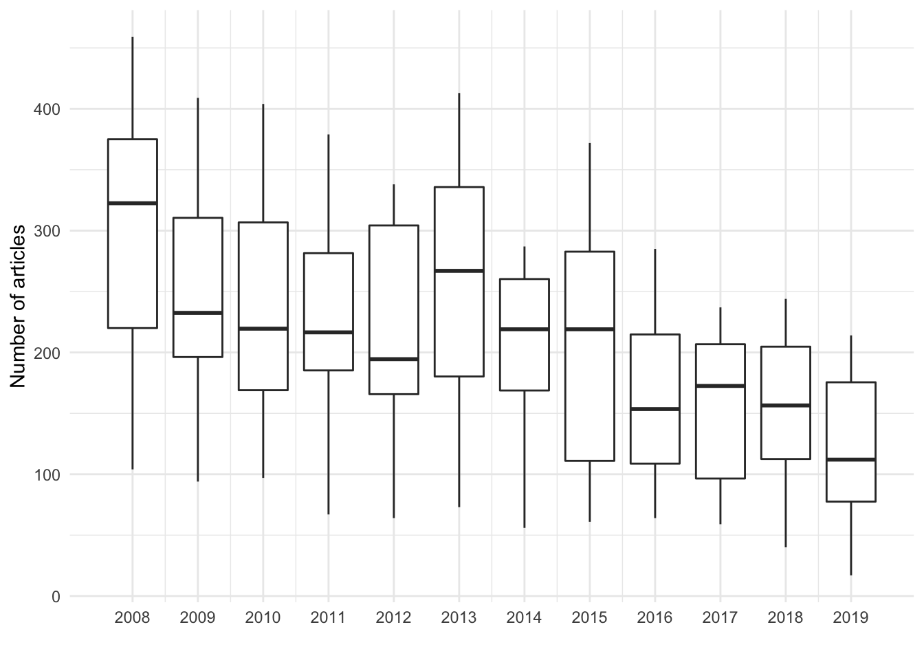
Figure 3: Boxplot of articles by year. The overall number of articles featuring the terms seems to decrease with time.
CQP-web vs metadata-annotated and Python-quantitated word counts
When carrying out modelling, it is often important to use data normalised to article word counts. This is dependent upon getting a correct word count for each article. Below, we compare article word counts from CQPWeb to those generated by Python and reported in the metadata in Lexis, for the condition-first language dataset as an example. The effects seen here will be consisten across other datasets as well.
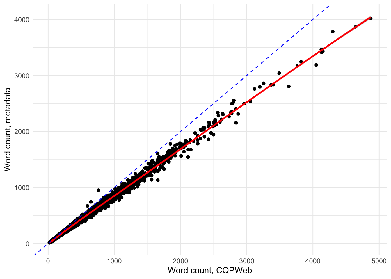
First, compare the counts from Python and the metadata:
Code
p<-condition_first_annotated%>%ggplot(aes(x =wordcount_total,
y =wordcount_from_metatata))+geom_point()+geom_smooth(method ="loess", formula =y~x, col ="red")+geom_abline(slope =1, intercept =0, col ="blue", lty =2)+xlab("Word count, Python")+ylab("Word count, metadata")plotly::ggplotly(p)
Figure 4: Correlation between word counts derived from the Lexis-supplied metadata and generated via Python counting. The correlation seems to be near-perfect (blue dashed line shows perfect equality, red is line of best fit of data).
The word counts are well correlated across all text lengths.
Next, we compare the word counts from CQP-web and the metadata:
Code
p<-condition_first_annotated%>%ggplot(aes(x =no_words_in_text,
y =wordcount_from_metatata))+geom_point()+geom_abline(slope =1, intercept =0, col ="blue", lty =2)+xlab("Word count, CQPWeb")+ylab("Word count, metadata")plotly::ggplotly(p)
Figure 5: Correlation between word counts derived from the Lexis-supplied metadata and reported by CQPweb. It appears that there is a strong overestimate of word counts by CQPweb.
We can see that the longer the text, the more the counts do not match what is in the metadata (or counted via Python). This is most likely to CQP-Web counting punctuation as tokens, thereby with longer text more punctuation is added to each text.
We can add a smoothed conditional means line (in red) to show the deviation between the identity line (y = x, shown dashed in blue) and the line of best fit:
Code
condition_first_annotated%>%ggplot(aes(x =no_words_in_text,
y =wordcount_from_metatata))+geom_point()+geom_smooth(method ="loess", formula =y~x, se =TRUE, col ="red")+geom_abline(slope =1, intercept =0, col ="blue", lty =2)+xlab("Word count, CQPWeb")+ylab("Word count, metadata")
Figure 6: Correlation between word counts derived from the Lexis-supplied metadata and reported by CQPweb. The blue dashed line shows perfect equality, red is line of best fit of data. The overestimate by CQPweb is clearly detectable.
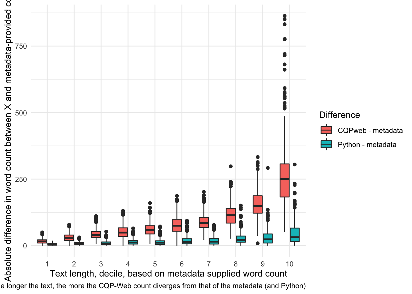
To make this more apparent, we plot the difference between the metadata-provided and Python and CQP-web counts:
Code
condition_first_annotated%>%mutate(
`Python - metadata` =(abs(wordcount_total-wordcount_from_metatata)),
`CQPweb - metadata` =(abs(no_words_in_text-wordcount_from_metatata)),
word_count_quartile =ntile(wordcount_from_metatata, 10))%>%select(`Python - metadata`, `CQPweb - metadata`, word_count_quartile)%>%pivot_longer(cols =c(`Python - metadata`, `CQPweb - metadata`))%>%ggplot(aes(x =as.factor(word_count_quartile),
y =value,
fill =name))+geom_boxplot()+labs(
x ="Text length, decile, based on metadata supplied word count",
y ="Absolute difference in word count between X and metadata-provided counts",
caption ="The longer the text, the more the CQP-Web count diverges from that of the metadata (and Python)")+guides(fill=guide_legend(title="Difference"))
Figure 7: Boxplot of absolute difference between (Python-metadata) and (CQPweb-metadata) derived word counts. It’s clear that the longer the text, the more CQPweb overestimates the word count, especially for the top decile of texts by length.
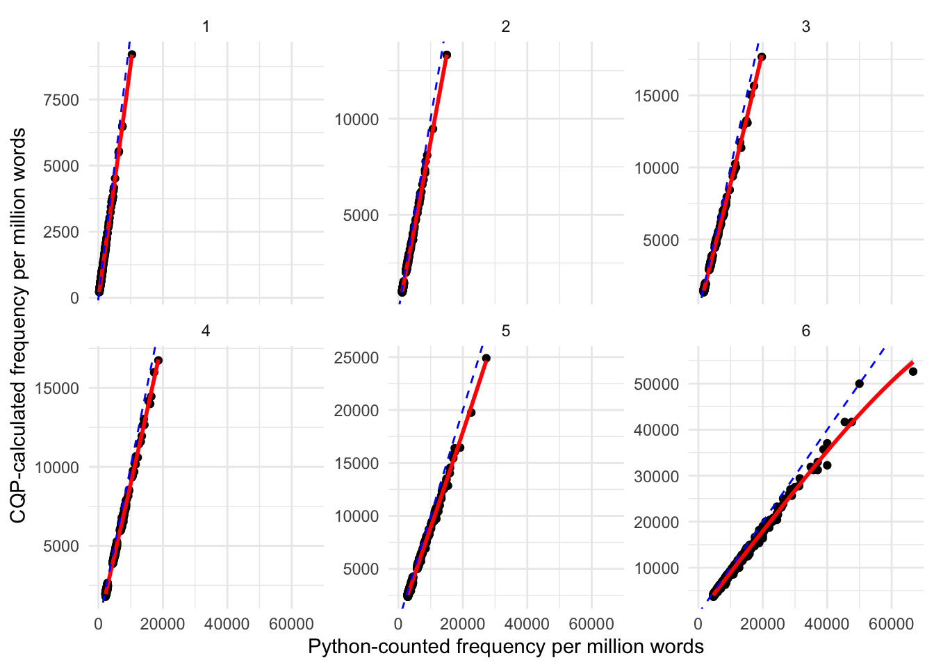
This also affects the normalised counts. To show this, we have broken the dataset into 6 groups based on text length, with 1 being the shortest and 6 being the longest texts. We can see that for the ~500 longest texts (panel 6), the line of best fit between frequencies is curved, showcasing how the normalised frequency is under-estimated for longer texts (due to the denominator for normalisation being bigger, as punctuation is included in the calculation).
Code
condition_first_annotated%>%mutate(frequency =10^6*no_hits_in_text/wordcount_total,
length_quantile =ntile(desc(condition_first_annotated$wordcount_total),6))%>%ggplot(aes(x =frequency, y =freq_per_million_words))+geom_point()+geom_smooth(method ="loess", formula =y~x, se =TRUE, col ="red")+geom_abline(slope =1, intercept =0, col ="blue", lty =2)+facet_wrap(~length_quantile, scales ="free_y")+labs(x ="Python-counted frequency per million words",
y ="CQP-calculated frequency per million words")
Figure 8: Comparison of effect of using CQPweb vs Python word counts by texts grouped into 6 length bins
CONCLUSION: Use the Python-generated total word count for calculating normalised frequencies (or the counts provided in the metadata, the two are nearly identical and well correlated across all text lengths. This also means we cannot use the provided normalised frequencies from CQPweb.