Data Wrangling
Overview
Teaching: 50 min
Exercises: 25 minQuestions
Tidyverse
Objectives
Introduction into tidyverse
Introduction into the grammar of tidyverse
Data wrangling

So far, we’ve been using R’s base functions to perform our data wrangling and manipulation.
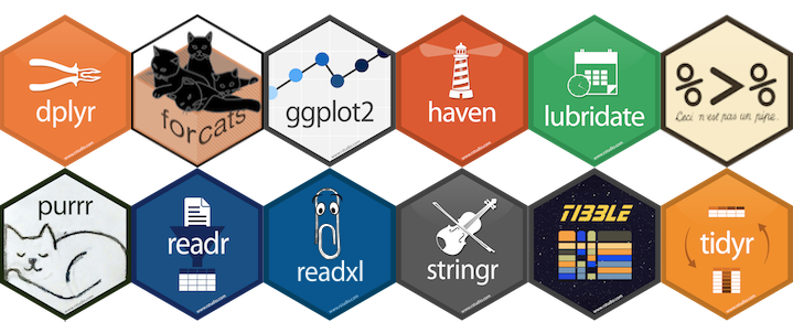
The advantage of working with R is that R has a large community of developers creating free and powerful tools (called libraries) which we can use. This includes the latest data wrangling, visualisation, statistical testing and machine learning tools.
I would highly encourage you to learn to use the tidyverse collection of data wrangling and visualisation tools. These are excellent tools that allows you to write elegent, legible code that gets your data into the right shape prior to analysis.
# load tidyverse
library(tidyverse)
── Attaching packages ────────────────────────────────── tidyverse 1.2.1 ──
✔ ggplot2 3.1.0     ✔ purrr   0.2.5
✔ tibble  1.4.2     ✔ dplyr   0.7.7
✔ tidyr   0.8.2     ✔ stringr 1.3.1
✔ readr   1.1.1     ✔ forcats 0.3.0
── Conflicts ───────────────────────────────────── tidyverse_conflicts() ──
✖ dplyr::filter() masks stats::filter()
✖ dplyr::lag()    masks stats::lag()
autism.data <- read_csv("data/autism_pids.csv")
Parsed with column specification:
cols(
  .default = col_integer(),
  gender = col_character(),
  ethnicity = col_character(),
  jaundice = col_character(),
  autism = col_character(),
  country = col_character(),
  used_app_before = col_character(),
  age_desc = col_character(),
  relation = col_character(),
  Class.ASD = col_character(),
  pids = col_character()
)
See spec(...) for full column specifications.
Next, we’ll step into one of the most popular tidyverse package called dplyr.
dplyr

dplyr allows you to perform some of the most common data manipulation tasks you’ll encounter in R. The background of the dplyr package is that it is a “grammar” of data manipulation and that its functions are a set of verbs.
You will also notice that the spelling follows British spelling rather than American (Hadley Wickham, author and maintainer of the tidyverse, is from New Zealand), but they can actually be used interchangeably. For example, summarise() and summarize() perform the same function.
select()
The select() function allows you to pick or remove variables based on their names. Note that you do not use " nor ' to wrap the column names as you would with a base R function
# select just the age, gender and result columns from autism.data (and rename country on the fly)
selected.autism.data <- select(autism.data, age, gender, result, country = country)
head(selected.autism.data)
# A tibble: 6 x 4
    age gender result country
  <int> <chr>   <int> <chr>
1    26 f           6 United States
2    24 m           5 Brazil
3    27 m           8 Spain
4    35 f           6 United States
5    40 f           2 Egypt
6    36 m           9 United States
# select all columns except for ethnicity and country
selected.autism.data <- select(autism.data, -ethnicity, -country)
head(selected.autism.data)
# A tibble: 6 x 21
     id A1_Score A2_Score A3_Score A4_Score A5_Score A6_Score A7_Score
  <int>    <int>    <int>    <int>    <int>    <int>    <int>    <int>
1     1        1        1        1        1        0        0        1
2     2        1        1        0        1        0        0        0
3     3        1        1        0        1        1        0        1
4     4        1        1        0        1        0        0        1
5     5        1        0        0        0        0        0        0
6     6        1        1        1        1        1        0        1
# ... with 13 more variables: A8_Score <int>, A9_Score <int>,
#   A10_Score <int>, age <int>, gender <chr>, jaundice <chr>,
#   autism <chr>, used_app_before <chr>, result <int>, age_desc <chr>,
#   relation <chr>, Class.ASD <chr>, pids <chr>
The tidyverse allows you to pipe functions together to create a chain to data manipulations. This allows you to redirect the output of one function into another one. Those familiar with bash or *nix will be familiar with piping with |. Here, we use %>% to pipe.
This makes each step discrete and helps immensely with readability. Also reduces your need to create temporary variables.
autism.data %>% select(age, gender, result) %>% head()
# A tibble: 6 x 3
    age gender result
  <int> <chr>   <int>
1    26 f           6
2    24 m           5
3    27 m           8
4    35 f           6
5    40 f           2
6    36 m           9
Or let’s make this more legible
autism.data %>%
  select(age, gender, result) %>%
  head()
# A tibble: 6 x 3
    age gender result
  <int> <chr>   <int>
1    26 f           6
2    24 m           5
3    27 m           8
4    35 f           6
5    40 f           2
6    36 m           9
Redirect the output of this chain of pipes into a new dataframe
autism.data %>%
  select(age, gender, result) -> selected.autism.data
filter()
The filter() function allows you to filter rows of your dataset that match some condition. We can also combine this with some of R’ base functions. Here, we’ll use head() to restrict the output number of rows
# get the first 6 people who are over 17
autism.data %>%
  filter(age == 17) %>%
  head()
# A tibble: 6 x 23
     id A1_Score A2_Score A3_Score A4_Score A5_Score A6_Score A7_Score
  <int>    <int>    <int>    <int>    <int>    <int>    <int>    <int>
1     7        0        1        0        0        0        0        0
2    10        1        1        1        1        0        1        1
3    13        0        1        1        1        1        1        0
4    14        1        0        0        0        0        0        1
5    15        1        0        0        0        0        0        1
6    85        1        1        0        0        0        0        0
# ... with 15 more variables: A8_Score <int>, A9_Score <int>,
#   A10_Score <int>, age <int>, gender <chr>, ethnicity <chr>,
#   jaundice <chr>, autism <chr>, country <chr>, used_app_before <chr>,
#   result <int>, age_desc <chr>, relation <chr>, Class.ASD <chr>,
#   pids <chr>
Combine this with the select() function to select only the age, gender and country of the 17 year olds in the autism dataset
autism.data %>%
  filter(age == 17) %>%
  select(age, gender, country) %>%
  head()
# A tibble: 6 x 3
    age gender country
  <int> <chr>  <chr>
1    17 f      United States
2    17 m      Bahamas
3    17 f      Bahamas
4    17 m      Austria
5    17 f      Argentina
6    17 f      New Zealand
What are the counts for countries of the 17 year olds in the autism dataset
autism.data %>%
  filter(age == 17) %>%
  select(country) %>%
  table()
.
           Argentina              Austria              Bahamas
                   1                    1                    2
              Canada                India          Netherlands
                   1                    1                    1
         New Zealand              Romania United Arab Emirates
                   4                    1                    1
      United Kingdom        United States
                   1                    4
arrange()
The arrange() function allows you to reorder the rows of your dataset
autism.data %>%
  arrange(age) %>%
  select(pids,age,  gender, Class.ASD) %>%
  head()
# A tibble: 6 x 4
  pids           age gender Class.ASD
  <chr>        <int> <chr>  <chr>
1 PatientID_7     17 f      NO
2 PatientID_10    17 m      YES
3 PatientID_13    17 f      NO
4 PatientID_14    17 m      NO
5 PatientID_15    17 f      NO
6 PatientID_85    17 f      NO
# If you want to arrange in reverse order it's also possible
autism.data %>%
  arrange(desc(age)) %>%
  select(pids,age,  gender, Class.ASD) %>%
  head()
# A tibble: 6 x 4
  pids            age gender Class.ASD
  <chr>         <int> <chr>  <chr>
1 PatientID_8      64 m      NO
2 PatientID_432    61 m      YES
3 PatientID_496    61 f      NO
4 PatientID_204    60 f      YES
5 PatientID_449    59 m      YES
6 PatientID_72     58 m      NO
mutate()
The mutate() function adds new columns for your data set
autism.data %>%
  mutate(result_squared = result^2) %>%
  select(pids, result, result_squared) %>%
  head()
# A tibble: 6 x 3
  pids        result result_squared
  <chr>        <int>          <dbl>
1 PatientID_1      6             36
2 PatientID_2      5             25
3 PatientID_3      8             64
4 PatientID_4      6             36
5 PatientID_5      2              4
6 PatientID_6      9             81
Section quiz
Output a table (do not create an object) with data only for female patients older than 30, with the columns pids, age, Class.ASD, result and scaled_result, where scaled_result is equal to age divided by result. Arrange this table by the scaled_result column in descending order.
Solution
autism.data %>%
filter(age > 30 & gender == "f") %>%
select(pids, age, gender, Class.ASD, result) %>%
mutate(scaled_result = age/result) %>%
arrange(desc(scaled_result))
You can also use mutate() to remove or edit existing columns
autism.data %>%
  mutate(age_desc = NULL, # this is to remove the age_desc column
         result = result + 1, # edit the existing result column
         agerank = rank(age)) %>% # add a new column called agerank
  select(-ends_with("Score")) %>% #show nifty feature to use select to remove multiple columns at one with ends_with
  head()
# A tibble: 6 x 13
     id   age gender ethnicity jaundice autism country used_app_before
  <int> <int> <chr>  <chr>     <chr>    <chr>  <chr>   <chr>
1     1    26 f      White-Eu… no       no     United… no
2     2    24 m      Latino    no       yes    Brazil  no
3     3    27 m      Latino    yes      yes    Spain   no
4     4    35 f      White-Eu… no       yes    United… no
5     5    40 f      <NA>      no       no     Egypt   no
6     6    36 m      Others    yes      no     United… no
# ... with 5 more variables: result <dbl>, relation <chr>,
#   Class.ASD <chr>, pids <chr>, agerank <dbl>
haven (interlude)

haven is a package within the tidyverse that allows you to read in data from SAS, SPSS and STATA. For example, if our autism dataset was saved as an .sav file (SPSS), we can use haven to read that in.
# load haven
library(haven)
autism.data.spss <- read_spss("data/autism_data.sav")
autism.data.spss <- autism.data.spss %>% mutate(ethnicity = na_if(ethnicity, "NA"),
                            age = na_if(age, "?"))
summarise() and group_by()
The summarise() function reduces down multiple values into one summary statistic. To do so, we need to tell R which groups we’re interested in summarising our data into. To do so, we need to use the group_by() function prior to calling summarise()
autism.data %>%
  group_by(Class.ASD) %>%
  summarise(meanage = mean(age, na.rm = TRUE),
            count = n())
# A tibble: 2 x 3
  Class.ASD meanage count
  <chr>       <dbl> <int>
1 NO           28.4   514
2 YES          31.3   189
You can group by more than one variable
autism.data %>%
  group_by(Class.ASD, gender) %>%
  summarise(mean.age = mean(age, na.rm = TRUE),
            max.age = max(age, na.rm = TRUE),
            min.age = min(age, na.rm = TRUE),
            count = n())
# A tibble: 4 x 6
# Groups:   Class.ASD [?]
  Class.ASD gender mean.age max.age min.age count
  <chr>     <chr>     <dbl>   <dbl>   <dbl> <int>
1 NO        f          28.7      61      17   233
2 NO        m          28.1      64      17   281
3 YES       f          31.3      60      17   103
4 YES       m          31.3      61      17    86
Section quiz
Create a summary table for mean ‘result’ after grouping by gender, autism class and family history of autism
Do the same as Q1 and now arrange from the lowest mean ‘result’ to the highest
Solution
- Despite the word of the question, we will first ‘group_by’ and then ‘summarise’
autism.data %>%
  group_by(gender, Class.ASD, autism) %>%
  summarise(mean.result = mean(result))
- We need to add in an ‘arrange’ at the end of our command
autism.data %>%
  group_by(gender, Class.ASD, autism) %>%
  summarise(mean.result = mean(result)) %>%
  arrange(mean.result)
Homework
You will need to refer to the tidyverse/dplyr help documentation to complete these exercises. We still refer to them on a daily basis even though we’ve been using these libraries for year - so this really is best practice for working with R.
- Create a table of number of patients by whether or not they’ve used the app before for each of the countries. (Hint: you will need to use the count() function for this).
- Is the average (mean) age of men or women greater in this dataset? Use group_by() and summarise() to find out
- In which country is the mean age of autism suffers highest?
- In which country is the mean age of parents who are also ASD suffers highest?
Key Points
R has a large community of developers creating power tools for data analysis
Tidyverse is a great data wrangling suite of functions
Use haven to read in your SPSS, STATA, etc files
Use dplyr to perform the common data manipulations