R variables and data types: Introduction to R Programming
Overview
Teaching: 40 min
Exercises: 20 minQuestions
R data types that will be useful in your own work
Objectives
Assign values to objects in R.
Solve simple arithmetic operations in R.
Describe what a data frame is.
R variables and data types
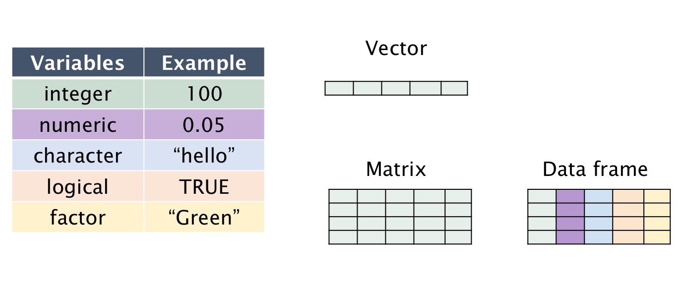
First, we introduce the common variable types and data types that you’ll be working with in R. Commonly, errors involve using the wrong variable or data type
| Variable type | Type | Example |
|---|---|---|
| integer | Whole numbers | 1, 100, -9 |
| numeric | Decimals | 0.1, -0.09, 234.567 |
| character | Text | “A”, “hello”, “welcome” |
| logical | Booleans | TRUE or FALSE |
| factor | Categorical | “green”, “blue”, “red”, “purple” |
| missing | Logical | NA |
| empty | - | NULL |
| Data type | Type |
|---|---|
| vector | 1D collection of variables of the same type |
| matrix | 2D collection of variables of the same type |
| data.frame | 2D collection of variables of multiple types |
Getting Started
Working directory
We’ve created this project in a “working directory”. To check where this is, use:
getwd()
[1] "/Users/nicholasho/Projects/workshops/sih_bmc_r_workshop_2018/lessonbmc/_episodes_rmd"
Calculating things in R
Standard math functions work in R:
2+3
[1] 5
1/1000
[1] 0.001
sqrt(2)
[1] 1.414214
We can store values in variables. Variables are a way to both store data and to label data.
myvariable <- 3
myvariable
[1] 3
myvariable = 3
myvariable
[1] 3
3 -> myvariable
myvariable
[1] 3
myvariable^2
[1] 9
Variable and Data Types
There are several different types of data you can use in R. We’ll examine a few common ones in a little more detail.
Text
Strings are known as “character” in R. Use the double quotes " or single quotes ' to wrap around the string
myname <- "nick"
We can use the class() function to see what data type it is
class(myname)
[1] "character"
Numbers
Numbers have different classes. The most common two are integer and numeric. Integers are whole numbers:
favourite.integer <- as.integer(8)
print(favourite.integer)
[1] 8
class(favourite.integer)
[1] "integer"
Numbers can be numeric which are decimals:
favourite.numeric <- as.numeric(8.8)
print(favourite.numeric)
[1] 8.8
class(favourite.numeric)
[1] "numeric"
pvalue.threshold <- 0.05
Logical (True/False)
We use the == to test for equality in R
class(TRUE)
[1] "logical"
favourite.numeric == 8.8
[1] TRUE
favourite.numeric == 9.9
[1] FALSE
Vectors
We can create 1D data structures called “vectors”.
1:10
[1] 1 2 3 4 5 6 7 8 9 10
2*(1:10)
[1] 2 4 6 8 10 12 14 16 18 20
seq(0, 10, 2)
[1] 0 2 4 6 8 10
We can store vectors and perform operations on them.
myvector <- 1:10
myvector
[1] 1 2 3 4 5 6 7 8 9 10
2^myvector
[1] 2 4 8 16 32 64 128 256 512 1024
b <- c(3,4,5)
b^2
[1] 9 16 25
disorders <- c("autism","ocd", "depression", "ocd", "anxiety", "autism")
disorders
[1] "autism"     "ocd"        "depression" "ocd"        "anxiety"
[6] "autism"
Automatic type conversions
R tries to be helpful by converting data to the same type within a vector when adding elements to a vector. This can result in unexpected problems…
mybool <- c(rep(TRUE, 5), rep(FALSE, 5))
class(mybool)
[1] "logical"
mybool <- c(mybool, 10)
class(mybool)
[1] "numeric"
mybool <- c(mybool, "10")
class(mybool)
[1] "character"
Factors
Factors store categorical data. Under the hood, factors are actually integers that have a string label attached to each unique integer. For example, if we have a long list of Male/Female labels for each of our patients, this will be stored a “row” of zeros and ones by R.
disorders <- as.factor(disorders)
class(disorders)
[1] "factor"
How many categories are there for disorders and what are they?
levels(disorders)
[1] "anxiety" "autism" "depression" "ocd"
nlevels(disorders)
[1] 4
A factor can be ordered. This makes sense in the context of a ranking such as a survey response, e.g. from ‘Strongly agree’ to ‘Strong disagree’.
responses <- c("low", "high", "medium", "low", "low", "high", "high", "medium", "medium")

myfactor <- factor(responses, levels = c("low", "medium", "high"))

myorderedfactor <- factor(responses, levels = c("low", "medium", "high"), ordered = TRUE)

levels(myfactor)
[1] "low" "medium" "high"
By default, factors will be ordered in alphabetical order.
Now our factor is ordered, we can find the lowest category by using min()
min(myfactor) #this will fail
Error in Summary.factor(structure(c(1L, 3L, 2L, 1L, 1L, 3L, 3L, 2L, 2L: 'min' not meaningful for factors
min(myorderedfactor)
[1] low
Levels: low < medium < high
Working with data
A lot of the time in R, we are working with tables of data, which are stored in a special data structure called R “data frames”.
Commonly,
rows should represent instances or individual observations e.g. data points, patients, events, samples, etc. while
columns will represent different types of data associated with each data point or instance e.g. Name, ID, location, time, value…
It is good practive to have a single row for every instance, and an individual, distinct measurement in each of the columns (not multiple measurements in one or redunant information in multiple columns). This is called tidy data, and makes it a lot easier to work with data frames. It’s also the source for the name “tidyverse”, which is a suite of packages we’ll be making extensive use of in the next few weeks to work with our data.
Here is an example data frame:
bmc.data <- data.frame(fname = c("Alice", "Bob", "Carol", "David"),
                       gender = as.factor(c("Female", "Male", "Female", "Male")),
                       disorder = c("autism", "anxiety", "autism", "depression"),
                       age = c(20, 45, 15, 12),
                       biomarker1 = c(5.70, 4.96, 1.37, 10.44),
                       clinicalstage = c("1b", "1a", "1a", "2"),
                       stringsAsFactors = FALSE)
Viewing The Data
Use the function View() to visually inspect the data in a new RStudio pane:
View(bmc.data)
How many rows and columns do we have?
nrow(bmc.data)
[1] 4
ncol(bmc.data)
[1] 6
dim(bmc.data)
[1] 4 6
Accessing Subsets
Return the first N rows of your data frame
head(bmc.data)
  fname gender   disorder age biomarker1 clinicalstage
1 Alice Female     autism  20       5.70            1b
2   Bob   Male    anxiety  45       4.96            1a
3 Carol Female     autism  15       1.37            1a
4 David   Male depression  12      10.44             2
The default for the head() function is to show the first 6 rows. How do we know this? Type ? infront of the function name in your console
?head
Return the first 3 rows of your data frame
head(bmc.data, n = 3)
  fname gender disorder age biomarker1 clinicalstage
1 Alice Female   autism  20       5.70            1b
2   Bob   Male  anxiety  45       4.96            1a
3 Carol Female   autism  15       1.37            1a
head(bmc.data, 3)
  fname gender disorder age biomarker1 clinicalstage
1 Alice Female   autism  20       5.70            1b
2   Bob   Male  anxiety  45       4.96            1a
3 Carol Female   autism  15       1.37            1a
bmc.data[1:3, ]
  fname gender disorder age biomarker1 clinicalstage
1 Alice Female   autism  20       5.70            1b
2   Bob   Male  anxiety  45       4.96            1a
3 Carol Female   autism  15       1.37            1a
bmc.data[c(1, 2, 3), ]
  fname gender disorder age biomarker1 clinicalstage
1 Alice Female   autism  20       5.70            1b
2   Bob   Male  anxiety  45       4.96            1a
3 Carol Female   autism  15       1.37            1a
bmc.data[c(TRUE, TRUE, TRUE, FALSE), ]
  fname gender disorder age biomarker1 clinicalstage
1 Alice Female   autism  20       5.70            1b
2   Bob   Male  anxiety  45       4.96            1a
3 Carol Female   autism  15       1.37            1a
As you can see, there are multiple ways to achieve the same result in R; this is very powerful for advanced users, but can be quite confusing for newcomers, since it’s not always clear what a particular chunk of code is doing.
Return the last 2 rows in a data set
tail(bmc.data, 2)
  fname gender   disorder age biomarker1 clinicalstage
3 Carol Female     autism  15       1.37            1a
4 David   Male depression  12      10.44             2
Return the “age” column in the data set
bmc.data$age
[1] 20 45 15 12
bmc.data[, 4]
[1] 20 45 15 12
bmc.data[, "age"]
[1] 20 45 15 12
Return only the first 3 rows and columns 2 and 5 of the data set
bmc.data[1:3, c(2,5)]
  gender biomarker1
1 Female       5.70
2   Male       4.96
3 Female       1.37
Return the columns named “fname” and “biomarker1”
bmc.data[,c("fname", "biomarker1")]
  fname biomarker1
1 Alice       5.70
2   Bob       4.96
3 Carol       1.37
4 David      10.44
Filtering the data
Return only the rows (patients) who are Female
bmc.data[bmc.data$gender == "Female", ]
  fname gender disorder age biomarker1 clinicalstage
1 Alice Female   autism  20       5.70            1b
3 Carol Female   autism  15       1.37            1a
What exactly happened here? We made a vector of TRUE/FALSE statements, for each row in which this condition is true and then we subset rows in which the index is true
females <- bmc.data$gender == "Female"
females
[1] TRUE FALSE TRUE FALSE
bmc.data[females, ]
  fname gender disorder age biomarker1 clinicalstage
1 Alice Female   autism  20       5.70            1b
3 Carol Female   autism  15       1.37            1a
Another way to subset the patients is with the which() function. This returns the TRUE indices of a logical object.
females <- which(bmc.data$gender == "Female")
females
[1] 1 3
bmc.data[females, ]
  fname gender disorder age biomarker1 clinicalstage
1 Alice Female   autism  20       5.70            1b
3 Carol Female   autism  15       1.37            1a
bmc.data[which(bmc.data$gender == "Female"), ]
  fname gender disorder age biomarker1 clinicalstage
1 Alice Female   autism  20       5.70            1b
3 Carol Female   autism  15       1.37            1a
What if we want all patients older than 16 years of age?
bmc.data[bmc.data$age > 16, ]
  fname gender disorder age biomarker1 clinicalstage
1 Alice Female   autism  20       5.70            1b
2   Bob   Male  anxiety  45       4.96            1a
Adding records
Add a new row to the data set using the rbind() function:
new.person <- data.frame(fname = "Evelyn",
                         gender = "Female",
                         disorder = "anxiety",
                         age = 27,
                         biomarker1 = 40.8,
                         clinicalstage = "2")

bmc.data <- rbind(bmc.data, new.person)
Section quiz
Return those patients whose clinical stage is “1a”
Return those patients whose biomarker1 value is less than 6.7
Return just the first name of all patients older than 16 years of age
Solution
- Return those patients whose clinical stage is “1a”
bmc.data[bmc.data$clinicalstage == "1a",]
- Return those patients whose biomarker1 value is less than 6.7
bmc.data[bmc.data$biomarker1 < 6.7,]
- Return just the first name of all patients older than 16 years of age
bmc.data[bmc.data$age > 16,]$fname
bmc.data[bmc.data$age > 16,"fname"]
Key Points
R supports multiple variable types
Errors often result because of trying to perform an unsupported operation on a specific data type
Errors can be cryptic to interpret
We can use helper packages to import and filter data in R