2.2.1 Sample size and statistical power
Learning objectives
- Explain why statistical power is necessary to interpret analysis results
- Identify design-stage strategies to ensure a study is well-powered (replication, platform-appropriate minimum sampling, detectable effect sizes)
- Describe analysis-stage strategies for validating power
- Explain why omics requires its own statistical methods, rather than classical power calculations
Sections 2.1.1 through 2.1.3 addressed whether a measurement can be trusted: whether the platform is appropriate, whether samples are allocated to avoid confounding, and whether measurements are consistent and documented. This section addresses whether there are enough independent observations to detect the effect of interest. A study can satisfy every criterion in Module 2.1 and still fail to replicate if the sample size was insufficient.
Consideration 3: Statistical power
A study is powered when the sample size is sufficient to detect the effect of interest with a specified probability. In omics, power is routinely not estimated before sample collection. The number of samples needed is often determined by budget, availability, or convention instead. An underpowered study may produce findings with elevated false positive rates and poor reproducibility.
Consideration 3: The multiple-testing burden
Classical power calculations assume a single hypothesis. In omics studies, thousands to millions of features are tested simultaneously, and false discovery rate correction lowers the effective significance threshold for each one. A study powered for one well-characterised feature is not powered for the dataset. The multiple-testing burden is not a statistical technicality to manage at analysis — it is part of the sample size problem and has to be accounted for at design.
Consideration 3: Effect size and variability must be estimated
Sample size calculations require an effect size and a variance estimate. Neither has a default value, and neither can be derived from the power calculation itself. They must come from domain knowledge, comparable published studies, or pilot data. Using assumed or generic values produces a sample size estimate that describes a study different from the one being designed. This is the step most often skipped, and it is why sample sizes set by budget or convention so often fall short.
Consideration 8: The unit of replication
Only biological replicates — independent samples from the population — contribute to n. Technical replicates, subsamples, and pooled material do not. The unit has to be identified before a sample size can be calculated, because the calculation is counting independent observations of that unit. A study that misidentifies the unit will produce an n that describes a different study.
The unit of replication
A study's sample size is not simply the number of files, wells, cells, or measurements produced. It is the number of independent biological units being compared, such as patients, animals, cultures, or environmental samples. Before running our models it is important to recognise what counts as one independent unit.
Two common design choices can make the apparent sample number differ from the real number of independent units.
- Subsampling takes many measurements from one biological unit: thousands of cells from one donor, multiple vials from one water body.
- Pooling merges material from several biological units before measurement, so the pool represents an average rather than any individual.
When subsamples are treated as independent biological replicates, the apparent n is inflated. This is like asking one person the same survey question five times and claiming you surveyed five people, you have more measurements, but not more independent information about the population. This is called pseudoreplication. The result of this is that the statistical analysis assumes more independent observations than actually exist, producing inflated degrees of freedom and overconfident p-values.
The activity below uses a concrete sampling scenario to distinguish valid biological replication from pseudoreplication, and to apply that distinction to the power and sample size questions that follow.
Activity part 1: Valid replication or pseudoreplication?
A team wants to know whether microbial communities differ between freshwater and marine environments. Two sampling designs are proposed. Both produce six samples and cost the same to sequence.
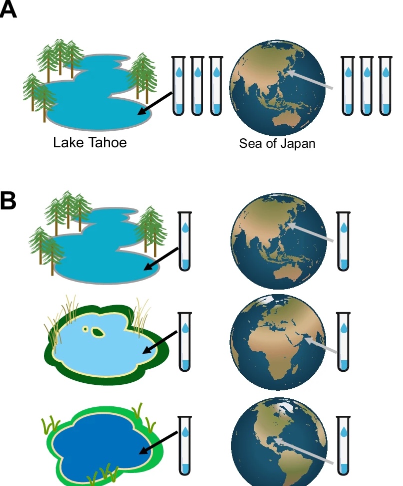
For panel A and then panel B:
- What is the biological unit the study wants to draw a conclusion about?
- What is the real n per environment?
- Is this valid biological replication, or pseudoreplication?
Wagner & Kleiner. Nature Communications 16, 7263 (2025). doi:10.1038/s41467-025-62616-x (CC BY-NC-ND 4.0)
Answer
Panel A is pseudoreplication. The biological unit is the water body. Three vials from the same lake are three observations of one lake, not three observations of freshwater. The real n is 1 per environment. Analysing the vials as n = 3 inflates degrees of freedom and produces a p-value for a comparison the study never made.
Panel B is valid replication. The real n is 3 per environment — one vial from each of three independently chosen bodies. The variation between the three lakes is the variation the question is about.
Panel A is not measuring nothing: it estimates within-body variability. It is not the quantity the research question asked for, and no analysis converts one into the other.
Statistical power in omics
Sample size in omics is rarely determined by a power calculation. It is determined by budget, sample availability, or instrument capacity, and is often fixed before anyone has asked what it takes to detect the effect of interest. The result is a study that is well-executed at the bench but underpowered for its bioinformatic analyses. A small sample size is not always obvious from the initial results. In fact, a study may still produce statistically significant findings, but those findings are more likely to be unstable, inflated in effect size, and difficult to replicate or validate.
Classical power calculations do not transfer directly to omics because the shape of the data is often reversed from the settings these formulas were built for. Many statistical workflows assume a relatively large number of observations and a smaller number of variables. Omics studies often have the opposite structure: relatively few samples, because data generation is expensive or the trait is rare, and a very large number of measured features, such as genes, proteins, metabolites, or genomic regions.
This matters because testing many features increases the occurance of false positives just by chance. Omics analyses therefore use false discovery rate correction, which makes the effective significance threshold more stringent for each feature. At the same time, different features vary by different amounts, and that variability is usually not known before the data are generated. A study powered to detect one well-characterised effect is therefore not necessarily powered for the full dataset. In practice, an analysis may return many possible signals before correction and far fewer after correction.
Multiple testing and false discovery rate correction
When a single hypothesis is tested at a 0.05 threshold, there is a 5% chance of a false positive. When 20,000 gene expression features are each tested at the same threshold, roughly 1,000 false positives are expected by chance alone, even if no true differences exist. Multiple testing correction addresses this by adjusting the significance threshold based on the number of tests performed.
The most widely used method in omics is Benjamini-Hochberg false discovery rate (FDR) correction, which controls the expected proportion of false positives among the features called significant. A 5% FDR means that 5% of reported findings are expected to be false positives. With more features tested and the same sample size, detecting true positives after correction requires larger effects or more samples. This is why a sample size adequate for a single-feature experiment is rarely adequate for an omics dataset.
Activity part 2: What does n = 3 mean for power?
Design B has n = 3 water bodies per environment. A 16S amplicon sequencing analysis will test thousands of microbial features simultaneously, with false discovery rate correction applied.
- Is n = 3 per environment likely to be sufficient for this analysis? What additional information would be needed to answer this properly?
- If the study fails to detect any significant differences after FDR correction, what are the possible explanations?
Answer
n = 3 per environment is likely insufficient for a well-powered analysis across thousands of features after FDR correction, but the specific answer depends on the expected effect size and the variability in microbial community composition between water bodies of the same type. Without those estimates, the power of the study cannot be determined — only that n = 3 is a low starting point by the standards of omics benchmarking studies.
If no significant differences are detected after FDR correction, there are two equally valid explanations: there is no genuine difference in microbial community composition between freshwater and marine environments, or the study was underpowered to detect a difference that exists. These cannot be distinguished from the data alone.
Estimating the sample size
A power calculation is a formula that estimates the sample size needed to detect an effect of a given magnitude, with a given probability, at a given significance threshold. It requires three inputs:
- Effect size: how large a difference is being detected
- Biological variability: how much samples differ from each other for reasons unrelated to the effect
- Multiple-testing burden: how many features are being tested and corrected simultaneously
None of these has a default value, and none can be derived from the calculation itself. They must be estimated before the calculation is run. In omics, where variance is feature-specific and rarely known in advance, sample size is best estimated empirically rather than calculated from assumed values.
The figure below illustrates how these two inputs interact. Each panel shows two populations being compared; the minimum sample size required to detect the difference changes substantially depending on how variable the measurements are within each group and how large the difference between groups is. High within-group variance or a small between-group difference both require more samples. When both conditions hold simultaneously, the required n rises sharply.
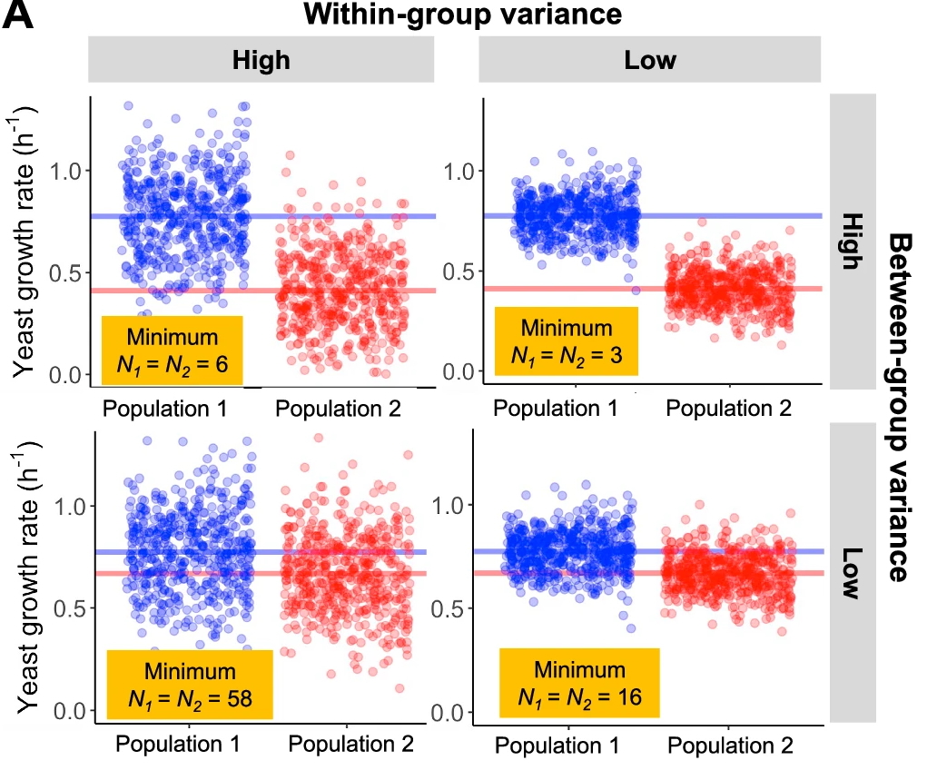
Wagner & Kleiner. Nature Communications 16, 7263 (2025). doi:10.1038/s41467-025-62616-x (CC BY-NC-ND 4.0)
Because the assumptions behind classical formulas rarely hold in omics, sample size is best estimated empirically from one or more of the following sources. Most studies should draw on more than one.
Three sources for effect size and variability estimates
Domain knowledge. What counts as a biologically meaningful difference is a scientific judgement before it is a statistical one. A twofold change may be routine in one system and implausible in another. Someone with working knowledge of the tissue, organism, or condition can usually bound the range of plausible effect sizes before any data are collected.
Comparable published studies. Work using the same platform, tissue, and comparison provides observed effect sizes and dispersion estimates from experiments already done. A published dataset that can be downloaded and measured directly is more informative than a reported summary statistic. Variability can differ substantially between tissues and platforms, so matching on both improves the estimate.
Pilot data. A small pilot dataset can be used to estimate variability directly, and the full analysis can then be simulated across a range of sample sizes. This carries realistic measurement noise into the estimate rather than assuming a variance that has not been observed.
Large benchmarking studies provide independent evidence of how sample size affects detection and reproducibility. Several have shown that n = 3 per group misses a substantial fraction of true differential signal. Any empirical estimate is more informative than a formula applied to a variance that was assumed.
Practical lower bounds
A note on practice
The approaches above describe what a well-powered study requires. In practice, sample size in omics is rarely determined this way. Budget constraints, limited sample availability, and fixed sequencing capacity mean that n is often set before any power estimate is run.
This does not make the estimate pointless, knowing the gap between the available sample size and the required one is itself informative. A study that is underpowered for its stated question can be reframed around what it is powered for, or the question can be narrowed to where the available n is sufficient. Running the estimate after the fact is better than not running it at all.
In addition to platform, the right sample size depends on four factors:
-
Biological variability: how much samples differ from each other for reasons unrelated to the effect of interest. Higher variability requires more samples to distinguish a true signal from background noise. This is the factor most likely to be underestimated at design stage, because it can only be known from pilot data or comparable published studies in the same tissue and system.
-
Effect size: how large a difference is expected between comparison groups. Larger effects require fewer samples to detect; subtle effects require many more. Effect size should be defined in biological terms (i.e. what magnitude of difference is meaningful for the question) before being translated into a statistical parameter.
-
Study design: the structure of the comparison determines the effective sample size available for each contrast. A two-group comparison with equal allocation uses samples efficiently; a multi-group or factorial design may require more total samples to maintain adequate power for each comparison of interest. Blocking and stratification (covered in module 2.1.2) can reduce variability and improve power without increasing n.
-
Discovery vs validation: discovery studies test many hypotheses simultaneously and tolerate a defined rate of false positives under FDR correction; validation studies typically test a smaller set of pre-specified hypotheses at a more stringent threshold. The same n that is adequate for discovery is rarely adequate for validation, because the significance threshold, the number of tests, and the tolerance for false positives all change.
Published lower bounds you come across in the literature (should) reflect the conditions of the studies that generated them: a specific tissue, organism, platform configuration, and effect size. A number that was adequate in one system may be inadequate in another with higher biological variability or a more subtle effect. These ranges are a starting point for the sample size conversation, not a threshold to clear.
| Layer | Platform(s) | How to determine n | Indicative range |
|---|---|---|---|
| Genome | WGS, WES | For variant calling: set sequencing depth first, then determine n based on variant frequency of interest. For association studies: use a GWAS power calculator with estimated allele frequency and effect size. For somatic calling: account for tumour purity in depth calculations. | Hundreds–thousands for association studies; rare variant studies require more |
| Epigenome | ChIP-seq, ATAC-seq, WGBS | Estimate from pilot data or comparable published datasets for the same tissue and antibody target. For WGBS, use a bisulfite-specific power tool with an estimate of the methylation difference expected. | ≥3 per condition for differential analysis; more when effect sizes are small |
| Transcriptome | Bulk RNA-seq | Use pilot data or a comparable public dataset to estimate dispersion, then simulate across a range of sample sizes using an RNA-seq power tool. | ≥6 per group for moderate–large effects; ≥12 when smaller effects matter |
| Transcriptome | scRNA-seq | Determine donor n and cell n separately. Donor n drives statistical power for between-group comparisons; use a power tool designed for multi-sample single-cell designs. | Donor n ≥6 per group as a starting point; cell number per donor is a secondary consideration |
| Proteome | Label-free MS | Anchor the calculation to the proteins the question depends on, accounting for expected missing value rate. Use a proteomics-specific sample size tool with pilot data where available. | No universal minimum; effective n per protein is lower than total samples run |
| Metabolome | LC-MS, GC-MS | Estimate from pilot data with the same collection protocol and pre-analytical conditions. Pre-analytical standardisation reduces variability and can improve power more than adding samples. | 5–10 per group for exploratory studies; substantially more for biomarker validation |
Activity part 3: How would you determine the right n?
The fieldwork budget allows for a maximum of 5 water bodies per environment. Before committing to this design, the team wants to know whether n = 5 is sufficient.
- What information is needed to run a power calculation for this study?
- Where would that information come from?
- If the estimate suggests n = 5 is underpowered, what are the options?
Answer
A power calculation requires an estimate of effect size (how different microbial community composition is expected to be between freshwater and marine environments) and biological variability (how much communities differ between water bodies of the same type). It also requires a decision about the significance threshold after FDR correction and the number of features being tested.
These estimates would come from published 16S studies comparing similar environment types, or from a small pilot dataset. Community composition variability between water bodies of the same type is the critical input — if it is high, more samples are needed to distinguish the freshwater/marine contrast from within-environment noise.
If n = 5 is underpowered, the options are: reduce the number of features tested (focus on a defined subset rather than the full community), accept lower power and frame the study as exploratory, or reframe the question around a contrast the available n is sufficient to detect.
Module 2.2.1 takeaways
- The n in a power calculation is the number of independent biological units.
- In omics studies, thousands of features are tested simultaneously, variance is feature-specific, and false discovery rate correction means that detecting true positives requires larger effects or more samples as the number of features increases.
- Effect size and variability must be estimated from domain knowledge, comparable published studies, or pilot data before the calculation is run. Any empirical estimate is more informative than a formula applied to an assumed variance.
- Published lower bounds reflect the conditions of the studies that produced them. They are a starting point, not a threshold to clear.
- When the available sample size falls short of what the question requires, the estimate still defines what the study is actually powered to detect, and the question can be scoped accordingly.