Exploratory Data Analysis (EDA)

Pima Indians Diabetes

Learning objective:

Use tidyverse functions for exploratory data analysis;
Introduce and explore the Pima Indians Diabetes dataset;
Impute missing data.

Today, we are going to be working with Pima Indian Women’s diabetes dataset which contains information on 768 Pima Indian women’s diabetes status, as well as many predictive features:

pregnant - Number of times pregnant
glucose - Plasma glucose concentration a 2 hours in an oral glucose tolerance test
pressure - Diastolic blood pressure (mm Hg)
triceps - Triceps skin fold thickness (mm) - a measure correlated with body fat
insulin - 2-Hour serum insulin (mu U/ml)
mass - Body mass index (weight in kg/(height in m)^2)
age - Age (years)
diabetes - diabetes status (pos - diabetic; neg - non-diabetic)
pedigree - diabetes pedigree function

The diabetes pedigree function was developed by Smith 1988 to provide a synthesis ofthe diabetes mellitus history in relatives and the genetic relationship of those relatives to the subject. It uses information from parents, grandparents, siblings, aunts and uncles, and first cousin to provide a measure of the expected genetic influence of affected and unaffected relatives on the subject’s eventual diabetes risk.

The Pima Indians are a group of Native Americans living in an area consisting of what is now central and southern Arizona. The short name, “Pima” is believed to have come from a phrase meaning “I don’t know,” which they used repeatedly in their initial meetings with Spanish colonists. Thanks Wikipedia!

Let’s Explore our data

library(tidyverse)
library(tidymodels)
library(ggcorrplot)
library(GGally)
library(qs)
library(mlbench)
library(skimr)
theme_set(theme_minimal())

Load data:

# load the Pima Indians dataset from the mlbench dataset
data(PimaIndiansDiabetes)
# rename dataset to have shorter name because lazy
diabetes_data <- PimaIndiansDiabetes
# look at the variable names
names(diabetes_data)

[1] "pregnant" "glucose"  "pressure" "triceps"  "insulin"  "mass"     "pedigree"
[8] "age"      "diabetes"

# look at the data
glimpse(diabetes_data)

Rows: 768
Columns: 9
$ pregnant <dbl> 6, 1, 8, 1, 0, 5, 3, 10, 2, 8, 4, 10, 10, 1, 5, 7, 0, 7, 1, 1…
$ glucose  <dbl> 148, 85, 183, 89, 137, 116, 78, 115, 197, 125, 110, 168, 139,…
$ pressure <dbl> 72, 66, 64, 66, 40, 74, 50, 0, 70, 96, 92, 74, 80, 60, 72, 0,…
$ triceps  <dbl> 35, 29, 0, 23, 35, 0, 32, 0, 45, 0, 0, 0, 0, 23, 19, 0, 47, 0…
$ insulin  <dbl> 0, 0, 0, 94, 168, 0, 88, 0, 543, 0, 0, 0, 0, 846, 175, 0, 230…
$ mass     <dbl> 33.6, 26.6, 23.3, 28.1, 43.1, 25.6, 31.0, 35.3, 30.5, 0.0, 37…
$ pedigree <dbl> 0.627, 0.351, 0.672, 0.167, 2.288, 0.201, 0.248, 0.134, 0.158…
$ age      <dbl> 50, 31, 32, 21, 33, 30, 26, 29, 53, 54, 30, 34, 57, 59, 51, 3…
$ diabetes <fct> pos, neg, pos, neg, pos, neg, pos, neg, pos, pos, neg, pos, n…

Look for missing data:

anyNA(diabetes_data)

[1] FALSE

It seems like there is no missing data.

Get a summary of the data frame:

summary(diabetes_data)

    pregnant         glucose         pressure         triceps     
 Min.   : 0.000   Min.   :  0.0   Min.   :  0.00   Min.   : 0.00  
 1st Qu.: 1.000   1st Qu.: 99.0   1st Qu.: 62.00   1st Qu.: 0.00  
 Median : 3.000   Median :117.0   Median : 72.00   Median :23.00  
 Mean   : 3.845   Mean   :120.9   Mean   : 69.11   Mean   :20.54  
 3rd Qu.: 6.000   3rd Qu.:140.2   3rd Qu.: 80.00   3rd Qu.:32.00  
 Max.   :17.000   Max.   :199.0   Max.   :122.00   Max.   :99.00  
    insulin           mass          pedigree           age        diabetes 
 Min.   :  0.0   Min.   : 0.00   Min.   :0.0780   Min.   :21.00   neg:500  
 1st Qu.:  0.0   1st Qu.:27.30   1st Qu.:0.2437   1st Qu.:24.00   pos:268  
 Median : 30.5   Median :32.00   Median :0.3725   Median :29.00            
 Mean   : 79.8   Mean   :31.99   Mean   :0.4719   Mean   :33.24            
 3rd Qu.:127.2   3rd Qu.:36.60   3rd Qu.:0.6262   3rd Qu.:41.00            
 Max.   :846.0   Max.   :67.10   Max.   :2.4200   Max.   :81.00

Exercise:

Look at the output of summary above and the table that explains what each of the variables are. Do the values make sense for all of: - (a) Pregnancies and Glucose - (b) Blood pressure and Skin thickness - (c) Insulin and DiabetesPedigreeFunction, and - (d) BMI and Age

If not, how do you think we should deal with them? Can you hypothesise what the consequences of this approach would be?

Solution

#Possibly missing: 

colSums(diabetes_data == 0)

pregnant  glucose pressure  triceps  insulin     mass pedigree      age 
     111        5       35      227      374       11        0        0 
diabetes 
       0

#Not missing:

colSums(diabetes_data != 0)

pregnant  glucose pressure  triceps  insulin     mass pedigree      age 
     657      763      733      541      394      757      768      768 
diabetes 
     768

It is clear that the values of several variables are zero when it is impossible for them to be so (i.e. this value could not be zero if it was measured). Hence, we are dealing with “hidden” missing data, and should recode it as NA.

The following variables have zero “values” that are actually likely to be missing:

Glucose (a)
BloodPressure (b)
SkinThickness (b)
Insulin (c)
BMI (d)

Let’s use visualisation to further explore the dataset

ggplot(diabetes_data, aes(x = pregnant, fill = diabetes)) + geom_bar(position = "dodge")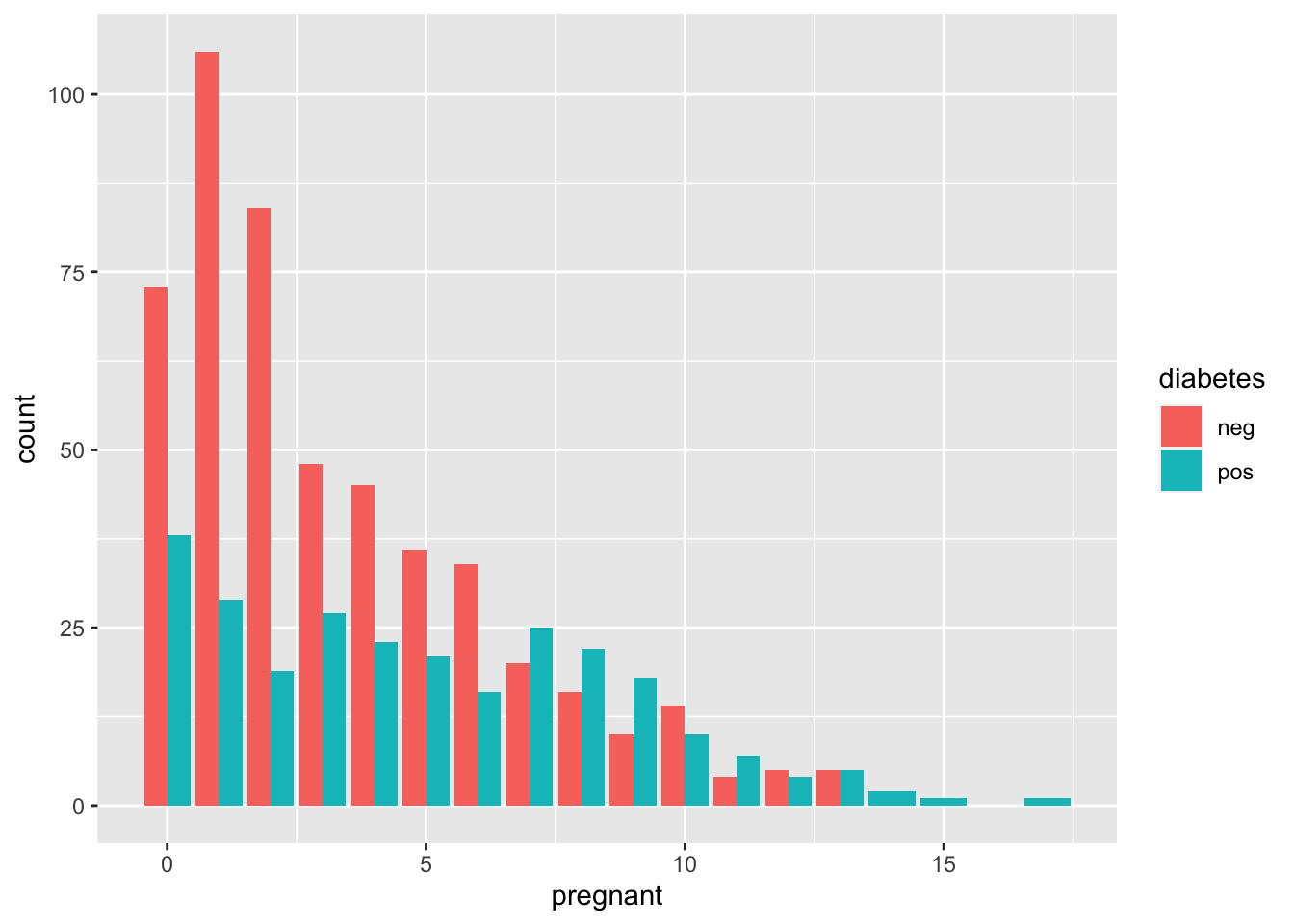

ggplot(
  diabetes_data,
  aes(
    x = pressure,
    y = glucose,
    color = diabetes
  )
) + geom_point(alpha = 0.5)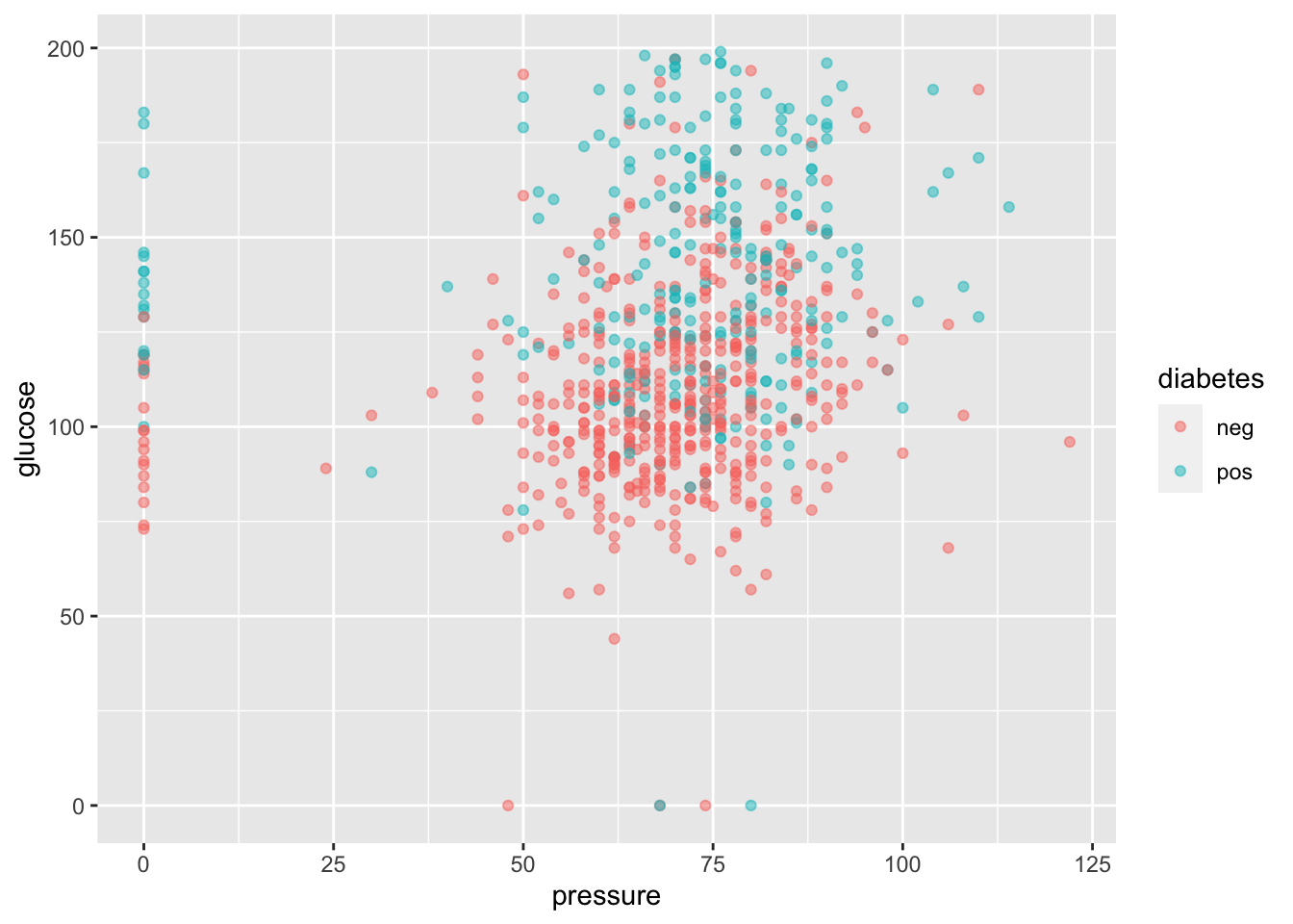

If we wanted to look at all possible scatterplot pairs we would do something like:

# make a pair plot
ggpairs(data = diabetes_data, 
        mapping = aes(color = diabetes),
        upper = list(combo = "box"))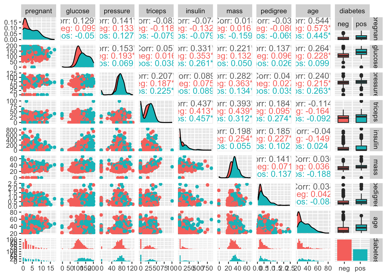

But it’s easier to look at a correlation plot:

# get a correlation matrix of the variables in the diabetes dataset:
diabetes_corr <- diabetes_data %>%
  # recode outcome to be numeric (subtract 1 to return it to zero/one)
  mutate(diabetes = as.integer(diabetes) - 1) %>%
  cor()

ggcorrplot(diabetes_corr, type = "lower", lab = TRUE )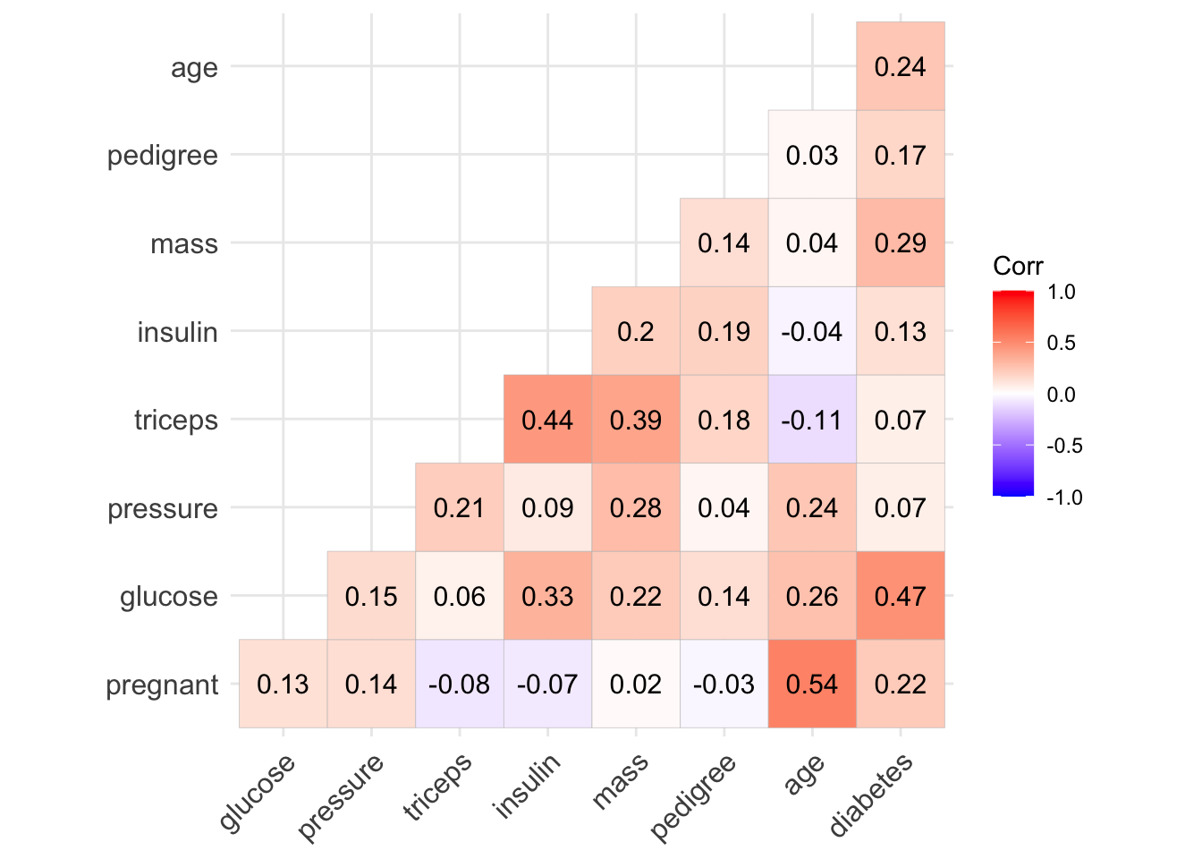

Let’s create a new dataframe d_na, which has the missing values recoded as NA:

d_na <- diabetes_data %>%
  mutate(glucose = na_if(glucose, 0)) %>%
  mutate(triceps = na_if(triceps, 0)) %>%
  mutate(insulin = na_if(insulin, 0)) %>%
  mutate(mass = na_if(mass, 0)) %>%
  mutate(pressure = na_if(pressure, 0))

# approximately half of the dataset is complete, whereas half is missing data
table(complete.cases(d_na))


FALSE  TRUE 
  376   392

naniar::gg_miss_var(d_na)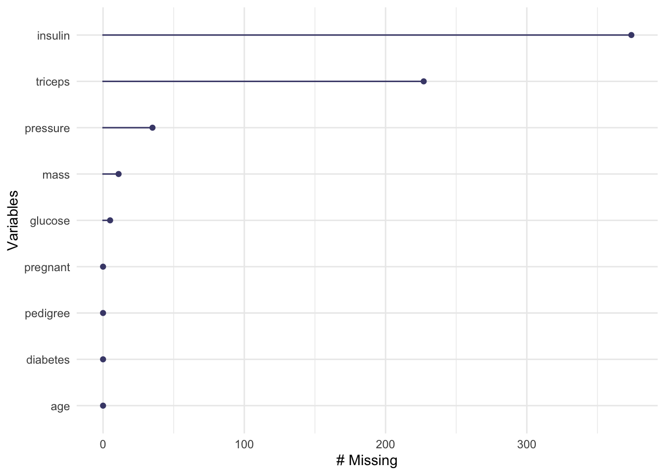

visdat::vis_dat(d_na)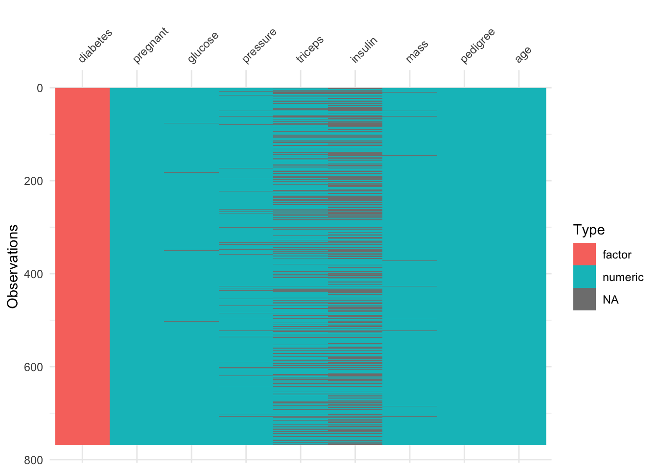

Let’s compare the correlation plot from before with another one now that we’ve correctly labelled the missing data:

diabetes_corr_na <-
  d_na %>%
  # recode outcome to be numeric (subtract 1 to return it to zero/one)
  mutate(diabetes = as.integer(diabetes) - 1) %>%
  # use pairwise complete observations for the two variables
  cor(use = "pairwise.complete.obs")

ggcorrplot(diabetes_corr_na,  type = "lower",lab = TRUE)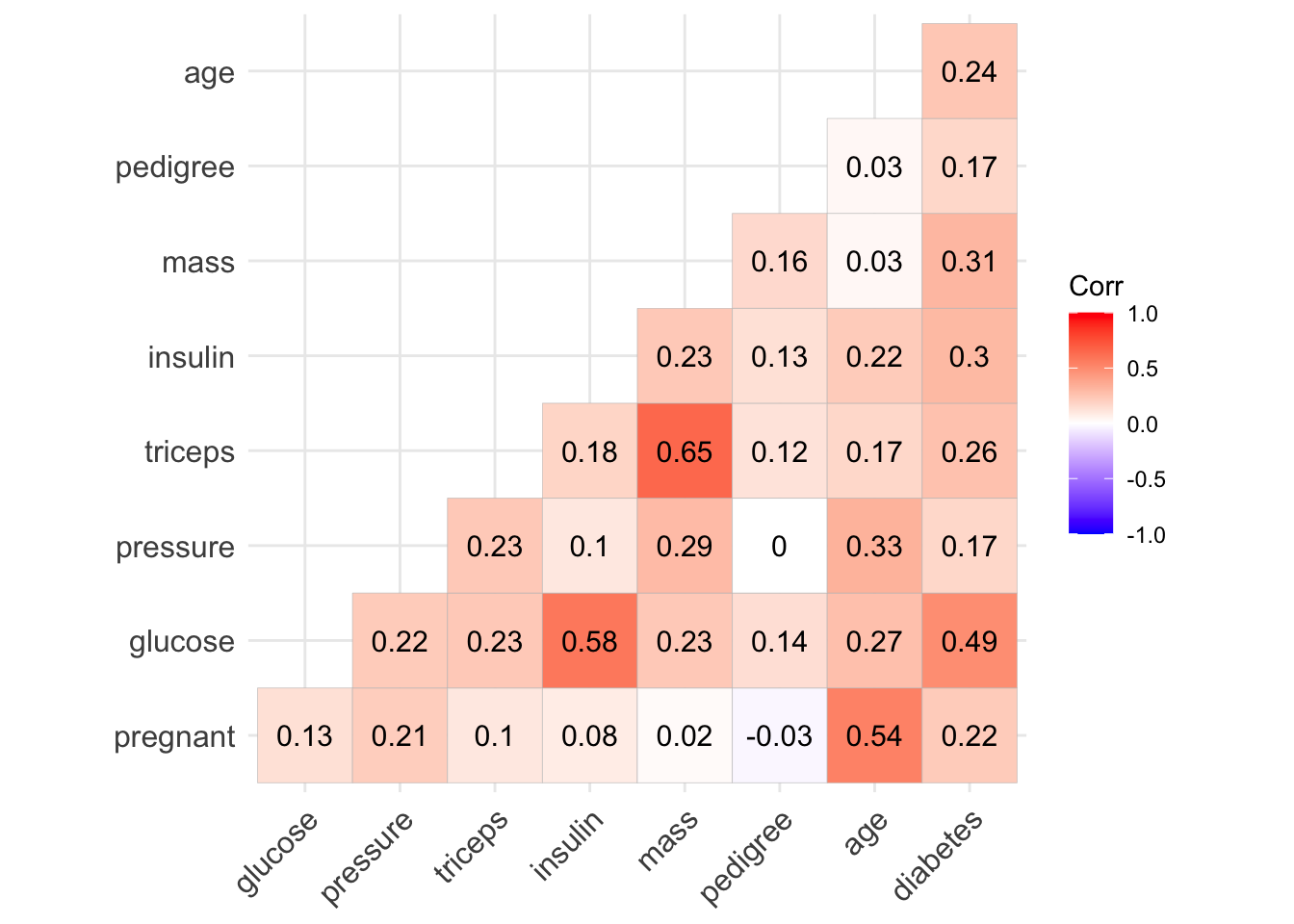

Notice that the correlation between some variables (eg. pregnant - insulin) changes quite substantially. (Negative before to Positive now).

Train-Test Split

We’re going to split our data into 70% training and 30% testing sets.

set.seed(42) # so we all get the same results

diabetes_split <- initial_split(d_na , prop = 0.7, strata = "diabetes" )
d_na_train <- training(diabetes_split)
d_na_test <- testing(diabetes_split)

qsave(d_na_train, "../_models/d_na_train.qs")
qsave(d_na_test, "../_models/d_na_test.qs")
qsave(diabetes_split, "../_models/diabetes_split.qs")

Some standard checks on the test/train split

Look how many examples we have in the training and testing sets.

dim(d_na_train)

[1] 537   9

dim(d_na_test)

[1] 231   9

Plot histograms of outputs to check we stratified appropriately

together <- bind_rows(train = d_na_train,
                      test = d_na_test,
                      .id = "test_train" ) 

together %>%
  ggplot(aes(x = diabetes))+
  geom_bar()+
  facet_grid(test_train~., scales = "free")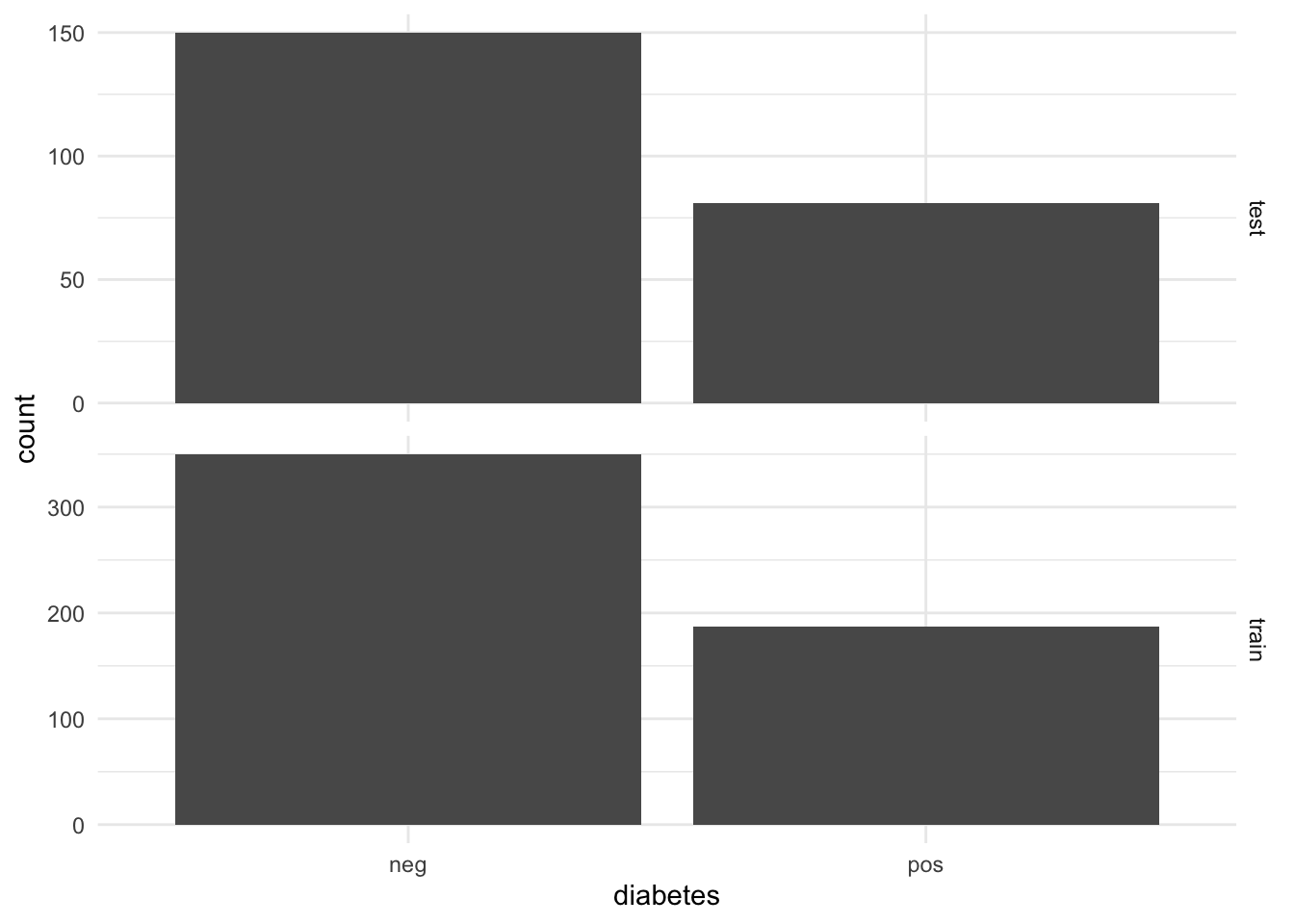

together %>%
  {ggduo(., 
         setdiff( names(.), c("test_train", "diabetes") ), 
         # column names not including test_train or the outcome
         "test_train")} # faceted by test_train split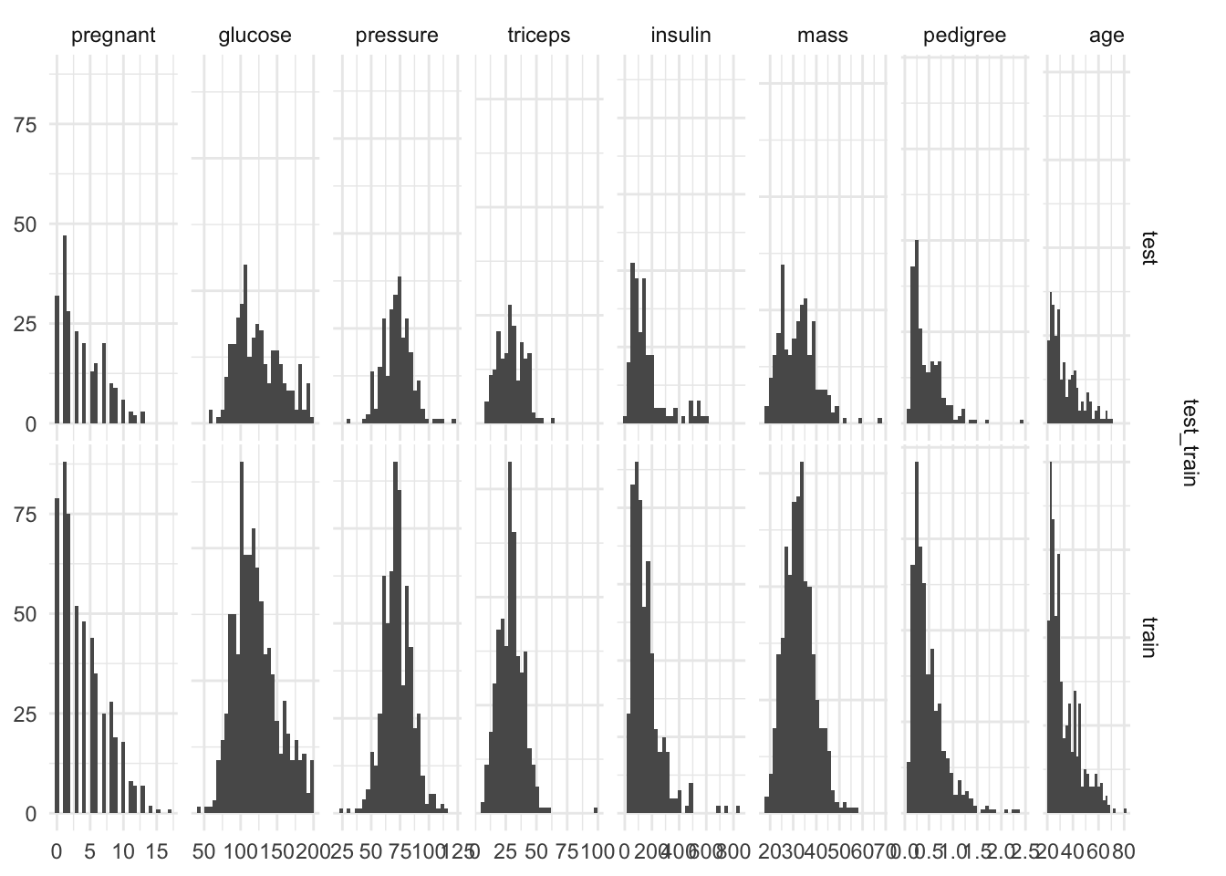

At some point we’re going to want to do some parameter tuning (explained later), and to do that we’re going to want to use cross-validation. So we can create a cross-validated version of the training set in preparation for that moment:

diabetes_folds <- vfold_cv(d_na_train, v=10, repeats = 5, strata = diabetes)

qsave(diabetes_folds, "../_models/diabetes_folds.qs")

Impute missing data

Imputation is often used to handle missing data because many statistical methods and machine learning algorithms require complete data. When we do imputation, we aren’t adding new information to our dataset, but we are using the patterns in our dataset so that we don’t have to throw away the data that have some variables missing. We can impute the missing data using a recipe:

# set seed to be 42 so everyone gets the same results
set.seed(42)

diabetes_rec <- recipe(diabetes ~ ., data = d_na_train) %>%
                step_impute_median(all_predictors()) %>%
                # all our predictors are numeric so standardize them
                step_normalize(all_numeric_predictors())
  

diabetes_rec  

qsave(diabetes_rec, "../_models/diabetes_rec.qs")

Key Points

Classification attempts to predict the class to which a particular observation belongs;
There are many different metrics for assessing performance for a classification problem;
Which metric you choose and optimise for should be considered carefully, and will be different depending on the problem;
Exporatory data analysis is a time consuming but critical process that needs to be carried out prior to any modeling.