Exploratory Data Analysis (EDA)
The Ames housing dataset
- Use Tidyverse functions for exploratory data analysis (EDA);
- Explore the Ames Housing dataset.
First, let’s load the required packages. We will use the tidyverse for general data processing and visualisation.
library(tidyverse)
library(naniar) # for visualising missing data
library(GGally) # for EDA
library(ggcorrplot)
library(AmesHousing)
library(plotly) # dynamic visualisations
library(bestNormalize)
library(qs)
library(janitor)
theme_set(theme_minimal())
We will use the Ames housing data to explore different ML approaches to regression. This dataset was “designed” by Dean De Cock as an alternative to the “classic” Boston housing dataset, and has been extensively used in ML teaching. It is also available from kaggle as part of its advanced regression practice competition.
The independent variables presented in the data include:
- 20 continuous variables relate to various area dimensions for each observation;
- 14 discrete variables, which typically quantify the number of items occurring within the house;
- 23 ordinal, 23 nominal categorical variables, with 2 (STREET: gravel or paved) - 28 (NEIGHBORHOOD) classes;
We will explore both the “uncleaned” data available from kaggle/UCI, and the processed data available in the AmesHousing package in R, for which documentation is available here. It can be useful for understanding what each of the independent variables mean.
ameshousing_temp <- AmesHousing::make_ames()

# Use this function to make the names easier to type
ameshousing <- ameshousing_temp %>%
  janitor::clean_names()

# Read in the uncleaned data.
ameshousing_uncleaned <- AmesHousing::ames_raw
Exploratory data analysis
Exploratory data analysis involves looking at:
- The distribution of variables in your dataset;
- Whether any data is missing;
- Data skewness;
- Correlated variables.
- Explore the Ames Housing dataset.
- What can you figure out about the different variables?
- Which do you think are more or less important?
- Compare the
ameshousingvariable, which is from the AmesHousing package in R and has been cleaned, with theameshousing_uncleaneddataset, which is the raw data from the UCI machine learning repository.- What was missing in the raw data?
- What are some of the approaches that have been taken to deal with missingness?
We can see that the “uncleaned” dataset has a lot of missing data, whereas it has been cleaned up for us in the “cleaned” one. In the interests of time, we will not focus here on how every variable in that dataset has been explored and cleaned up - however, it presents a good example of “messy” real-world data, so we would encourage you to try and look at a handful of variables at home, to see how they’ve been processed.
dim(ameshousing)[1] 2930 81glimpse(ameshousing)Rows: 2,930
Columns: 81
$ ms_sub_class <fct> One_Story_1946_and_Newer_All_Styles, One_Story_1946…
$ ms_zoning <fct> Residential_Low_Density, Residential_High_Density, …
$ lot_frontage <dbl> 141, 80, 81, 93, 74, 78, 41, 43, 39, 60, 75, 0, 63,…
$ lot_area <int> 31770, 11622, 14267, 11160, 13830, 9978, 4920, 5005…
$ street <fct> Pave, Pave, Pave, Pave, Pave, Pave, Pave, Pave, Pav…
$ alley <fct> No_Alley_Access, No_Alley_Access, No_Alley_Access, …
$ lot_shape <fct> Slightly_Irregular, Regular, Slightly_Irregular, Re…
$ land_contour <fct> Lvl, Lvl, Lvl, Lvl, Lvl, Lvl, Lvl, HLS, Lvl, Lvl, L…
$ utilities <fct> AllPub, AllPub, AllPub, AllPub, AllPub, AllPub, All…
$ lot_config <fct> Corner, Inside, Corner, Corner, Inside, Inside, Ins…
$ land_slope <fct> Gtl, Gtl, Gtl, Gtl, Gtl, Gtl, Gtl, Gtl, Gtl, Gtl, G…
$ neighborhood <fct> North_Ames, North_Ames, North_Ames, North_Ames, Gil…
$ condition_1 <fct> Norm, Feedr, Norm, Norm, Norm, Norm, Norm, Norm, No…
$ condition_2 <fct> Norm, Norm, Norm, Norm, Norm, Norm, Norm, Norm, Nor…
$ bldg_type <fct> OneFam, OneFam, OneFam, OneFam, OneFam, OneFam, Twn…
$ house_style <fct> One_Story, One_Story, One_Story, One_Story, Two_Sto…
$ overall_qual <fct> Above_Average, Average, Above_Average, Good, Averag…
$ overall_cond <fct> Average, Above_Average, Above_Average, Average, Ave…
$ year_built <int> 1960, 1961, 1958, 1968, 1997, 1998, 2001, 1992, 199…
$ year_remod_add <int> 1960, 1961, 1958, 1968, 1998, 1998, 2001, 1992, 199…
$ roof_style <fct> Hip, Gable, Hip, Hip, Gable, Gable, Gable, Gable, G…
$ roof_matl <fct> CompShg, CompShg, CompShg, CompShg, CompShg, CompSh…
$ exterior_1st <fct> BrkFace, VinylSd, Wd Sdng, BrkFace, VinylSd, VinylS…
$ exterior_2nd <fct> Plywood, VinylSd, Wd Sdng, BrkFace, VinylSd, VinylS…
$ mas_vnr_type <fct> Stone, None, BrkFace, None, None, BrkFace, None, No…
$ mas_vnr_area <dbl> 112, 0, 108, 0, 0, 20, 0, 0, 0, 0, 0, 0, 0, 0, 0, 6…
$ exter_qual <fct> Typical, Typical, Typical, Good, Typical, Typical, …
$ exter_cond <fct> Typical, Typical, Typical, Typical, Typical, Typica…
$ foundation <fct> CBlock, CBlock, CBlock, CBlock, PConc, PConc, PConc…
$ bsmt_qual <fct> Typical, Typical, Typical, Typical, Good, Typical, …
$ bsmt_cond <fct> Good, Typical, Typical, Typical, Typical, Typical, …
$ bsmt_exposure <fct> Gd, No, No, No, No, No, Mn, No, No, No, No, No, No,…
$ bsmt_fin_type_1 <fct> BLQ, Rec, ALQ, ALQ, GLQ, GLQ, GLQ, ALQ, GLQ, Unf, U…
$ bsmt_fin_sf_1 <dbl> 2, 6, 1, 1, 3, 3, 3, 1, 3, 7, 7, 1, 7, 3, 3, 1, 3, …
$ bsmt_fin_type_2 <fct> Unf, LwQ, Unf, Unf, Unf, Unf, Unf, Unf, Unf, Unf, U…
$ bsmt_fin_sf_2 <dbl> 0, 144, 0, 0, 0, 0, 0, 0, 0, 0, 0, 0, 0, 0, 1120, 0…
$ bsmt_unf_sf <dbl> 441, 270, 406, 1045, 137, 324, 722, 1017, 415, 994,…
$ total_bsmt_sf <dbl> 1080, 882, 1329, 2110, 928, 926, 1338, 1280, 1595, …
$ heating <fct> GasA, GasA, GasA, GasA, GasA, GasA, GasA, GasA, Gas…
$ heating_qc <fct> Fair, Typical, Typical, Excellent, Good, Excellent,…
$ central_air <fct> Y, Y, Y, Y, Y, Y, Y, Y, Y, Y, Y, Y, Y, Y, Y, Y, Y, …
$ electrical <fct> SBrkr, SBrkr, SBrkr, SBrkr, SBrkr, SBrkr, SBrkr, SB…
$ first_flr_sf <int> 1656, 896, 1329, 2110, 928, 926, 1338, 1280, 1616, …
$ second_flr_sf <int> 0, 0, 0, 0, 701, 678, 0, 0, 0, 776, 892, 0, 676, 0,…
$ low_qual_fin_sf <int> 0, 0, 0, 0, 0, 0, 0, 0, 0, 0, 0, 0, 0, 0, 0, 0, 0, …
$ gr_liv_area <int> 1656, 896, 1329, 2110, 1629, 1604, 1338, 1280, 1616…
$ bsmt_full_bath <dbl> 1, 0, 0, 1, 0, 0, 1, 0, 1, 0, 0, 1, 0, 1, 1, 1, 0, …
$ bsmt_half_bath <dbl> 0, 0, 0, 0, 0, 0, 0, 0, 0, 0, 0, 0, 0, 0, 0, 0, 0, …
$ full_bath <int> 1, 1, 1, 2, 2, 2, 2, 2, 2, 2, 2, 2, 2, 1, 1, 3, 2, …
$ half_bath <int> 0, 0, 1, 1, 1, 1, 0, 0, 0, 1, 1, 0, 1, 1, 1, 1, 0, …
$ bedroom_abv_gr <int> 3, 2, 3, 3, 3, 3, 2, 2, 2, 3, 3, 3, 3, 2, 1, 4, 4, …
$ kitchen_abv_gr <int> 1, 1, 1, 1, 1, 1, 1, 1, 1, 1, 1, 1, 1, 1, 1, 1, 1, …
$ kitchen_qual <fct> Typical, Typical, Good, Excellent, Typical, Good, G…
$ tot_rms_abv_grd <int> 7, 5, 6, 8, 6, 7, 6, 5, 5, 7, 7, 6, 7, 5, 4, 12, 8,…
$ functional <fct> Typ, Typ, Typ, Typ, Typ, Typ, Typ, Typ, Typ, Typ, T…
$ fireplaces <int> 2, 0, 0, 2, 1, 1, 0, 0, 1, 1, 1, 0, 1, 1, 0, 1, 0, …
$ fireplace_qu <fct> Good, No_Fireplace, No_Fireplace, Typical, Typical,…
$ garage_type <fct> Attchd, Attchd, Attchd, Attchd, Attchd, Attchd, Att…
$ garage_finish <fct> Fin, Unf, Unf, Fin, Fin, Fin, Fin, RFn, RFn, Fin, F…
$ garage_cars <dbl> 2, 1, 1, 2, 2, 2, 2, 2, 2, 2, 2, 2, 2, 2, 2, 3, 2, …
$ garage_area <dbl> 528, 730, 312, 522, 482, 470, 582, 506, 608, 442, 4…
$ garage_qual <fct> Typical, Typical, Typical, Typical, Typical, Typica…
$ garage_cond <fct> Typical, Typical, Typical, Typical, Typical, Typica…
$ paved_drive <fct> Partial_Pavement, Paved, Paved, Paved, Paved, Paved…
$ wood_deck_sf <int> 210, 140, 393, 0, 212, 360, 0, 0, 237, 140, 157, 48…
$ open_porch_sf <int> 62, 0, 36, 0, 34, 36, 0, 82, 152, 60, 84, 21, 75, 0…
$ enclosed_porch <int> 0, 0, 0, 0, 0, 0, 170, 0, 0, 0, 0, 0, 0, 0, 0, 0, 0…
$ three_season_porch <int> 0, 0, 0, 0, 0, 0, 0, 0, 0, 0, 0, 0, 0, 0, 0, 0, 0, …
$ screen_porch <int> 0, 120, 0, 0, 0, 0, 0, 144, 0, 0, 0, 0, 0, 0, 140, …
$ pool_area <int> 0, 0, 0, 0, 0, 0, 0, 0, 0, 0, 0, 0, 0, 0, 0, 0, 0, …
$ pool_qc <fct> No_Pool, No_Pool, No_Pool, No_Pool, No_Pool, No_Poo…
$ fence <fct> No_Fence, Minimum_Privacy, No_Fence, No_Fence, Mini…
$ misc_feature <fct> None, None, Gar2, None, None, None, None, None, Non…
$ misc_val <int> 0, 0, 12500, 0, 0, 0, 0, 0, 0, 0, 0, 500, 0, 0, 0, …
$ mo_sold <int> 5, 6, 6, 4, 3, 6, 4, 1, 3, 6, 4, 3, 5, 2, 6, 6, 6, …
$ year_sold <int> 2010, 2010, 2010, 2010, 2010, 2010, 2010, 2010, 201…
$ sale_type <fct> WD , WD , WD , WD , WD , WD , WD , WD , WD , WD , W…
$ sale_condition <fct> Normal, Normal, Normal, Normal, Normal, Normal, Nor…
$ sale_price <int> 215000, 105000, 172000, 244000, 189900, 195500, 213…
$ longitude <dbl> -93.61975, -93.61976, -93.61939, -93.61732, -93.638…
$ latitude <dbl> 42.05403, 42.05301, 42.05266, 42.05125, 42.06090, 4…colSums(is.na(ameshousing_uncleaned)) Order PID MS SubClass MS Zoning Lot Frontage
0 0 0 0 490
Lot Area Street Alley Lot Shape Land Contour
0 0 2732 0 0
Utilities Lot Config Land Slope Neighborhood Condition 1
0 0 0 0 0
Condition 2 Bldg Type House Style Overall Qual Overall Cond
0 0 0 0 0
Year Built Year Remod/Add Roof Style Roof Matl Exterior 1st
0 0 0 0 0
Exterior 2nd Mas Vnr Type Mas Vnr Area Exter Qual Exter Cond
0 23 23 0 0
Foundation Bsmt Qual Bsmt Cond Bsmt Exposure BsmtFin Type 1
0 80 80 83 80
BsmtFin SF 1 BsmtFin Type 2 BsmtFin SF 2 Bsmt Unf SF Total Bsmt SF
1 81 1 1 1
Heating Heating QC Central Air Electrical 1st Flr SF
0 0 0 1 0
2nd Flr SF Low Qual Fin SF Gr Liv Area Bsmt Full Bath Bsmt Half Bath
0 0 0 2 2
Full Bath Half Bath Bedroom AbvGr Kitchen AbvGr Kitchen Qual
0 0 0 0 0
TotRms AbvGrd Functional Fireplaces Fireplace Qu Garage Type
0 0 0 1422 157
Garage Yr Blt Garage Finish Garage Cars Garage Area Garage Qual
159 159 1 1 159
Garage Cond Paved Drive Wood Deck SF Open Porch SF Enclosed Porch
159 0 0 0 0
3Ssn Porch Screen Porch Pool Area Pool QC Fence
0 0 0 2917 2358
Misc Feature Misc Val Mo Sold Yr Sold Sale Type
2824 0 0 0 0
Sale Condition SalePrice
0 0 colSums(is.na(ameshousing)) ms_sub_class ms_zoning lot_frontage lot_area
0 0 0 0
street alley lot_shape land_contour
0 0 0 0
utilities lot_config land_slope neighborhood
0 0 0 0
condition_1 condition_2 bldg_type house_style
0 0 0 0
overall_qual overall_cond year_built year_remod_add
0 0 0 0
roof_style roof_matl exterior_1st exterior_2nd
0 0 0 0
mas_vnr_type mas_vnr_area exter_qual exter_cond
0 0 0 0
foundation bsmt_qual bsmt_cond bsmt_exposure
0 0 0 0
bsmt_fin_type_1 bsmt_fin_sf_1 bsmt_fin_type_2 bsmt_fin_sf_2
0 0 0 0
bsmt_unf_sf total_bsmt_sf heating heating_qc
0 0 0 0
central_air electrical first_flr_sf second_flr_sf
0 0 0 0
low_qual_fin_sf gr_liv_area bsmt_full_bath bsmt_half_bath
0 0 0 0
full_bath half_bath bedroom_abv_gr kitchen_abv_gr
0 0 0 0
kitchen_qual tot_rms_abv_grd functional fireplaces
0 0 0 0
fireplace_qu garage_type garage_finish garage_cars
0 0 0 0
garage_area garage_qual garage_cond paved_drive
0 0 0 0
wood_deck_sf open_porch_sf enclosed_porch three_season_porch
0 0 0 0
screen_porch pool_area pool_qc fence
0 0 0 0
misc_feature misc_val mo_sold year_sold
0 0 0 0
sale_type sale_condition sale_price longitude
0 0 0 0
latitude
0 Visualise missingness
When working with missing data, it can be helpful to look for “co-missingness”, i.e. multiple variables missing together. For example, when working with patient data, number of pregnancies, age at onset of menstruation and menopause may all be missing - which, when observed together, may indicate that these samples come from male patients for whom this data is irrelevant. “Gender” may or may not be a variable coded in the dataset.
A way of visualising missing data in the tidy context has been proposed @tierney2018expanding. See this web page for more options for your own data.
Let’s look at the missing variables in our housing data:
gg_miss_var(ameshousing_uncleaned)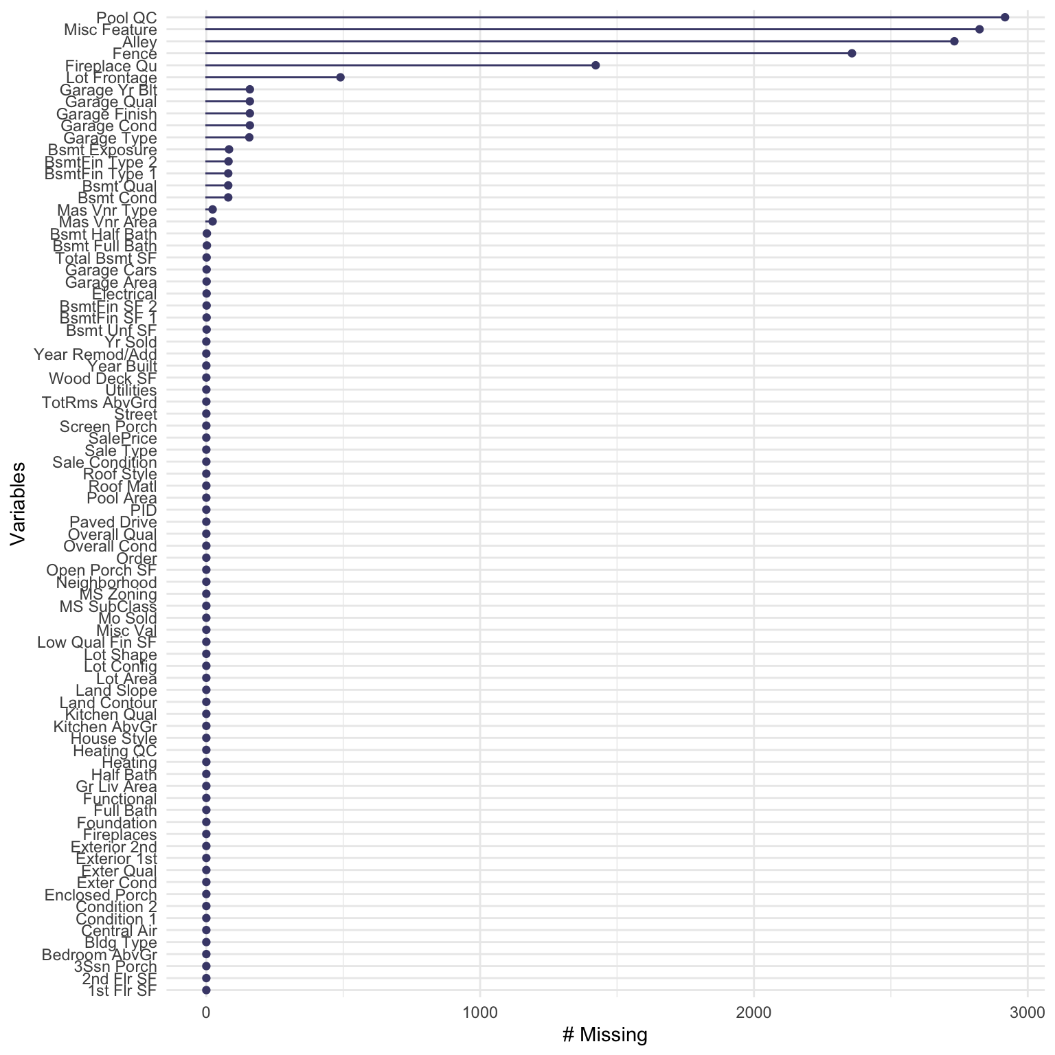
We can see that the most missingness is observed in the Pool_QC, Misc_Feature, Alley, Fence and Fireplace_QC variables. This is most likely due to many houses not having pools, alleys, fences, and fireplaces, and not having any features that the real estate agent considers to be notable enough to be added to the “miscellaneous” category.
An upset plot will give us more idea about the co-missingness of these variables:
gg_miss_upset(ameshousing_uncleaned, nsets = 10)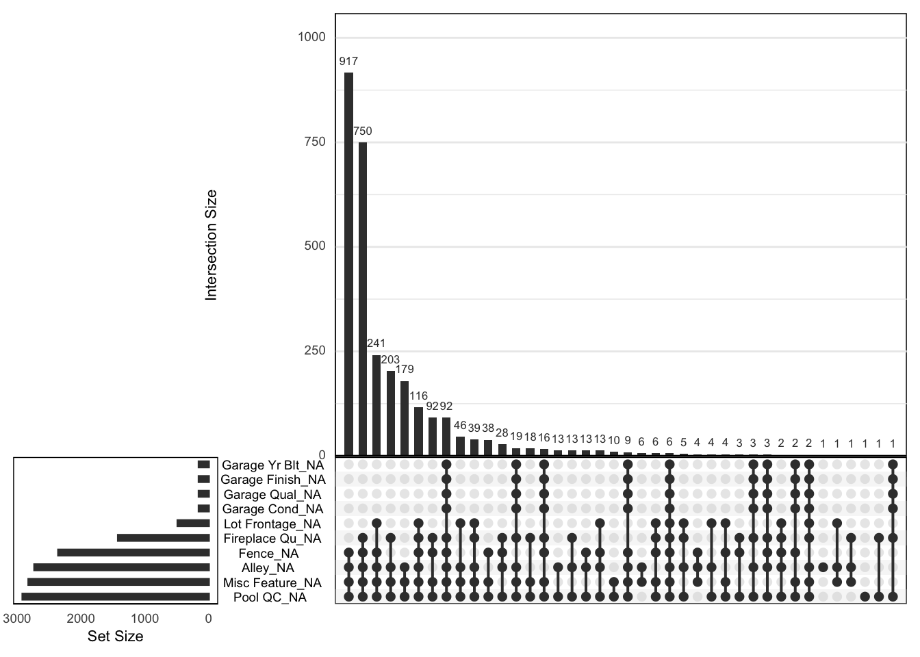
- Which variables are most frequently missing together?
- Does this “co-missingness” make sense?
Fence, alley, misc feature and pool qc are most often missing together. This probably means that a house doesn’t have an alley, a fence, a pool or any other miscellaneous features.
Similarly, the second most frequent “co-missingess” involves these plus missing “fireplace quality”, most likely due to the house not having fireplace.
We can also see that garage_yr_blt, garage_finish, garage_qual and garage_cond “co-miss” the same number of times - probably because these represent houses without garages.
Next, let’s create two “helper” vectors with the names of the numeric and categorical variables from the ameshousing dataset, which we can then use to batch subset our dataset prior to EDA/visualisation:
# pull out all of the numerical variables
numVars <- ameshousing %>%
  select_if(is.numeric) %>%
  names()

# use Negate(is.numeric) to pull out all of the categorical variables
catVars <- ameshousing %>%
  select_if(Negate(is.numeric)) %>%
  names()
Let’s then use the ggpairs() function to generate a plot of the first 10 numeric variables (and sale price, which is 33) against each other. We can repeat this for variables 11-20 and 21-33.
ggpairs(data = ameshousing,
        columns = numVars[c(1:10, 33)],
        title = "Numeric variables 1 - 10")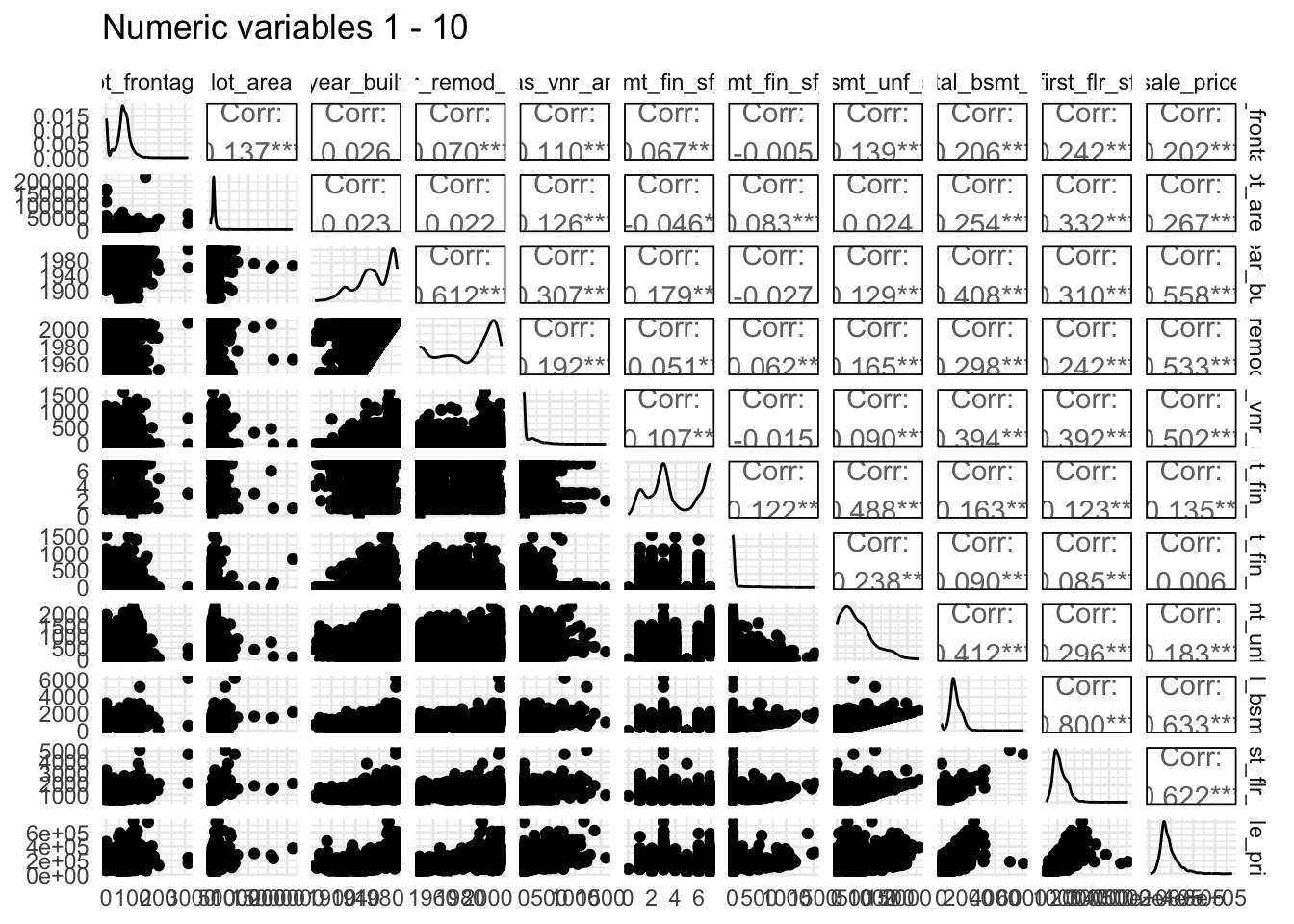
# ggpairs(ameshousing, numVars[c(11:20, 33)], title = "Numeric variables 11 - 20")
# ggpairs(ameshousing, numVars[c(21:33)], title = "Numeric variables 21 - 33")
ggpairs(data = ameshousing,
        columns = c(catVars[2:5], "sale_price"),
        title = "Some categorical variables")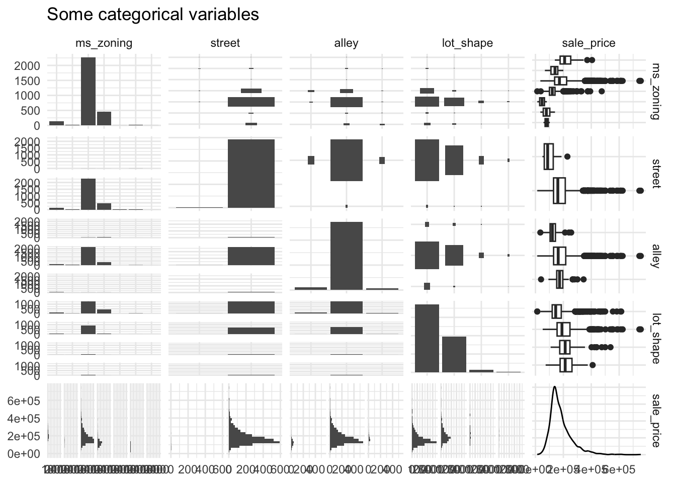
Next, we can generate a correlation plot between all of our numeric variables. By default, the cor() method will calculate the Pearson correlation between the Sale_Price and the other variables, and we can specify how we’d like to handle missing data when calculating this correlation.
In this case, we use pairwise.complete.obs, which calculates the correlation between each pair of variables using all complete pairs of observations on those variables.
We then plot the correlation using the corrplot library, which has several options for how to visualise a correlation plot. See here for some examples of the visualisations it can produce.
# pairs.panels(ameshousing[ , names(ameshousing)[c(3, 16, 23, 27,37)]], scale=TRUE)
ameshousingCor <- cor(ameshousing[,numVars],
                      use = "pairwise.complete.obs")

ameshousingCor_pvalues <- cor_pmat(ameshousingCor)
ggcorrplot(ameshousingCor, type = "lower")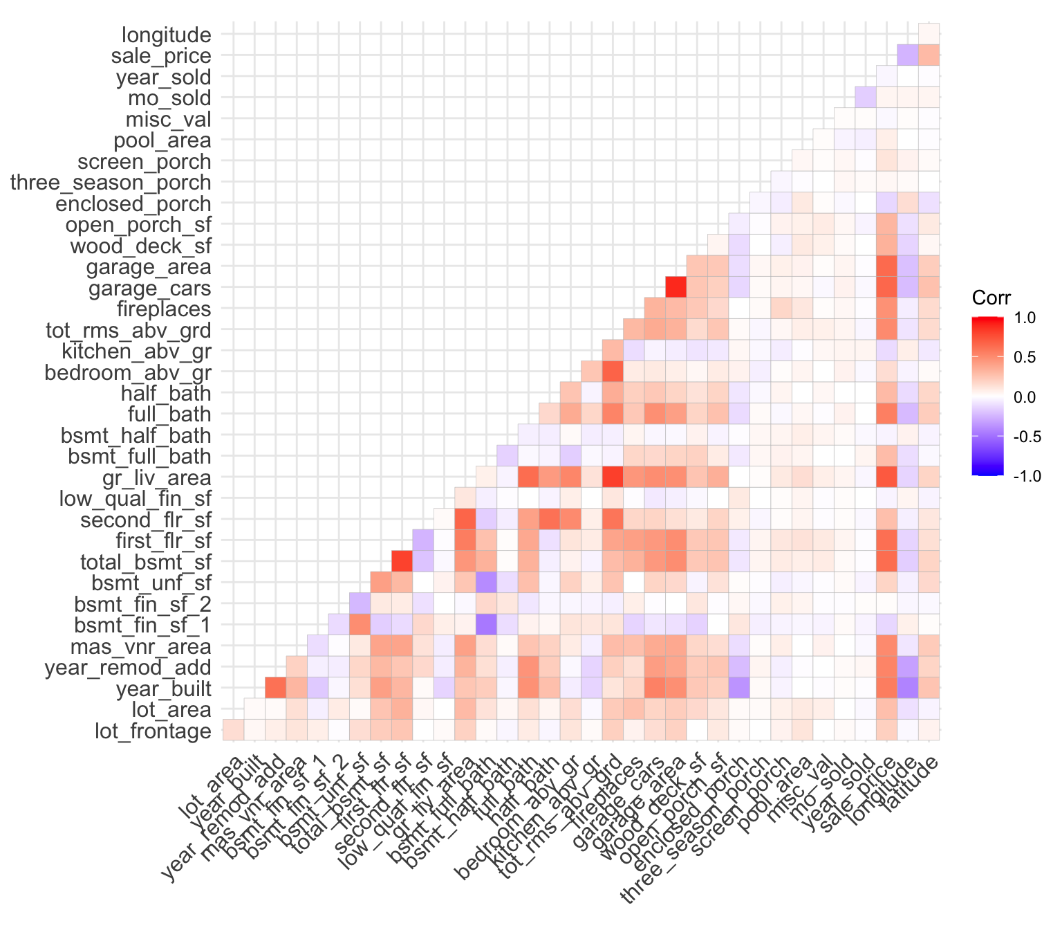
We can also make a dynamic visualisation using plotly.
#Bonus: interactive corrplot with zoom and mouseover
ggcorrplot(ameshousingCor, type = "lower") %>% ggplotly()- What variables are the most correlated with SalePrice?
as_tibble(ameshousingCor, rownames = "rowname") %>%
  gather(pair, value, -rowname) %>%
  filter(rowname != pair) %>% #remove self correlation
  filter(rowname == "sale_price") %>%
  arrange(desc(abs(value))) %>%
  head()
# A tibble: 6 × 3
rowname pair value
<chr> <chr> <dbl>
1 sale_price gr_liv_area 0.707
2 sale_price garage_cars 0.648
3 sale_price garage_area 0.640
4 sale_price total_bsmt_sf 0.633
5 sale_price first_flr_sf 0.622
6 sale_price year_built 0.558We can also plot this, using a slightly different representation:
- Circles instead of only colour to represent correlation levels
- Filter out correlations less than 0.5
all_numVar <- ameshousing[, numVars]
cor_numVar <- cor(all_numVar, use="pairwise.complete.obs")
CorHigh <- as_tibble(
  data.frame(correlation = cor_numVar[,'sale_price']), rownames = "rownames")  %>%
  filter(abs(correlation) >= 0.5) %>%
  .$rownames
ggcorrplot(cor_numVar[CorHigh, CorHigh], type = "lower", "circle")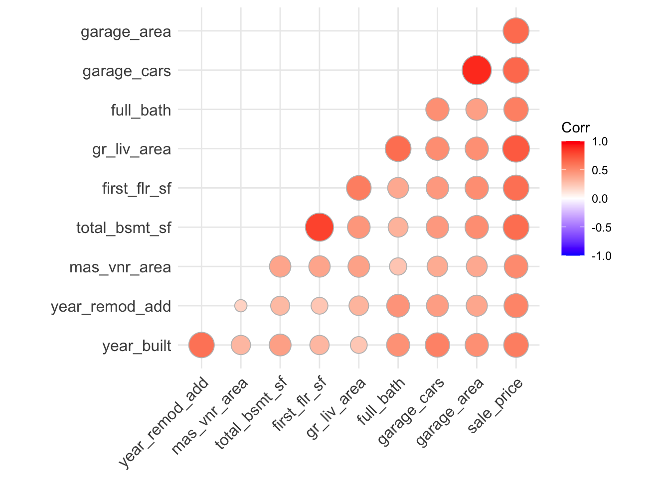
Let’s plot one of these relationships:
ameshousing %>%
  ggplot(aes(x = gr_liv_area, y = sale_price/1000)) +
  geom_point(alpha = 0.1) +
  labs(y = "Sale Price/$1000",
       x = "Living Area (sq.ft)",
       title = "Ames Housing Data") +
  geom_smooth(method= "lm")  +
  theme(axis.text.x = element_text(angle = 45, hjust = 1))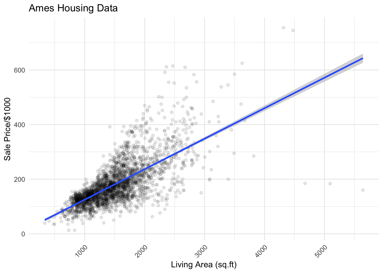
- How can we make our figures interactive?
- Using the
plotlypackage, we can turn anyggplot()object into an interactive plot usingplotly::ggplotly()
For example:
# First we save the ggplot as an object
plot <- ameshousing %>%
  ggplot(aes(x = gr_liv_area, y = sale_price / 1000)) +
  geom_point(alpha = 0.1) +
  labs(y = "Sale Price/$1000",
       x = "Living Area (sq.ft)",
       title = "Ames Housing Data") +
  geom_smooth(method = "lm")  +
  theme(axis.text.x = element_text(angle = 45, hjust = 1))

# then we pass it to ggplotly()
ggplotly(plot)
We can see that there are five houses with an area > 4000 square feet that seem to be outliers in the data. We should filter them out. Next, let’s generate a boxplot by Quality:
# Create a filtered dataframe
ameshousing_filt <-
  ameshousing %>%
  filter(gr_liv_area <= 4000)

# Make our ggplot object
p <- ameshousing_filt %>%
  mutate(quality = as.factor(overall_qual)) %>%
  ggplot(aes(x = quality,
             y = sale_price / 1000,
             fill = quality)) +
  labs(y = "Sale Price in $k's",
       x = "Overall Quality of House",
       title = "Ames Housing Data") +
  geom_boxplot() +
  theme(axis.text.x = element_text(angle = 45, hjust = 1))

# Now make it a plotly
ggplotly(p)
EDA of outcome variable
You also need to do EDA on the outcome variable to:
- identify outliers
- explore whether there is any skew in its distribution
- identify a transformation to use when modelling the data (if appropriate)
This is because many models, including ordinary linear regression, assume that prediction errors (and hence the response) are normally distributed.
ameshousing_filt %>%
  ggplot(aes(x = sale_price/1000)) +
  geom_histogram(bins = 50) +
  labs(x = "Sale Price in $k's",
       y = "Number of Houses sold")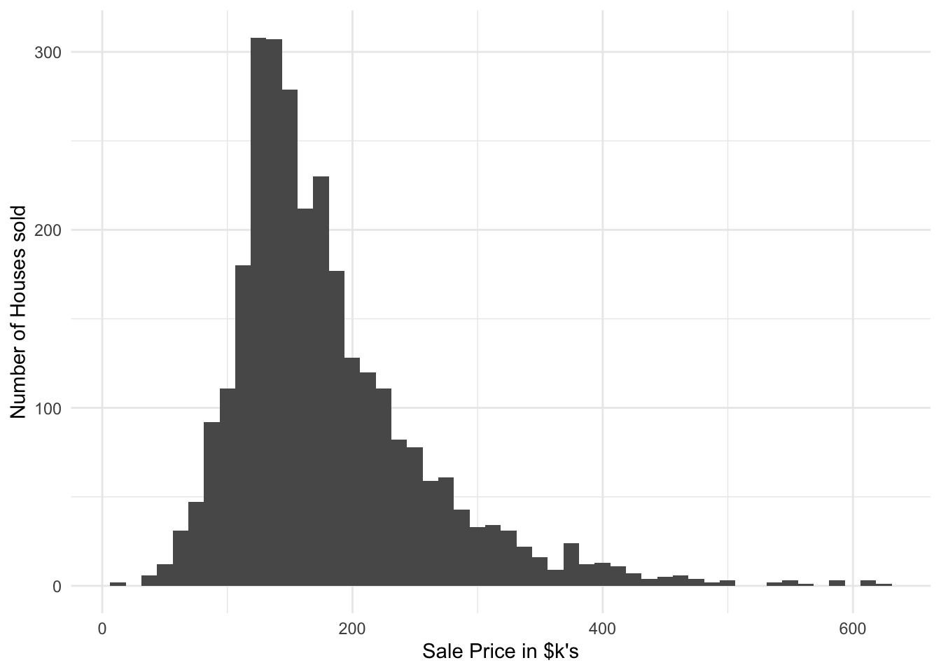
Let’s explore different ways of transforming the Sale Price.
#No transform

ameshousing_filt %>%
  ggplot(aes( sample = sale_price)) +
stat_qq() + stat_qq_line(col = "blue")![]()
#Sqrt transform

ameshousing_filt %>%
  ggplot(aes( sample = sqrt(sale_price))) +
stat_qq() + stat_qq_line(col = "blue")![]()
#natural log transform

ameshousing_filt %>%
  ggplot(aes( sample = log(sale_price))) +
stat_qq() + stat_qq_line(col = "blue")![]()
#log10 transform

ameshousing_filt %>%
  ggplot(aes( sample = log10(sale_price))) +
stat_qq() + stat_qq_line(col = "blue")![]()
- If you were working with this dataset, which of the above would you prefer?
The log10 transformation seems best, as it both helps the distribution look more normal and helps keep our error metrics and final predictions easily interpretable. It also means that the errors of predicting the values of inexpensive and expensive houses will affect the prediction equally.
bestNormalize::bestNormalize(
  ameshousing_filt$sale_price,
  allow_orderNorm = FALSE)
Best Normalizing transformation with 2925 Observations
Estimated Normality Statistics (Pearson P / df, lower => more normal):
- arcsinh(x): 1.6306
- Box-Cox: 1.6891
- Center+scale: 5.1734
- Double Reversed Log_b(x+a): 10.0059
- Log_b(x+a): 1.6306
- sqrt(x + a): 2.8254
- Yeo-Johnson: 1.6932
Estimation method: Out-of-sample via CV with 10 folds and 5 repeats
Based off these, bestNormalize chose:
Standardized asinh(x) Transformation with 2925 nonmissing obs.:
Relevant statistics:
- mean (before standardization) = 12.71303
- sd (before standardization) = 0.4060161 The bestNormalize library can be used to identify the best normalising transformation. Note that in this case, the arcsinh(x) and logarithmic transformations both achieve best normalisation results. To make interpretation a bit easier, we choose the logarithmic transformation.
ameshousing_filt$sale_price <- log10(ameshousing_filt$sale_price)Feature transformation
The year in which the house was built and the year when it was remodelled are not really the most relevant parameters we look at when buying a house: instead, buyers usually care a lot more about the age of the house and the time since the last remodel. Let’s transform these features:
ameshousing_filt_tr <-
  ameshousing_filt %>%
  mutate(time_since_remodel = year_sold - year_remod_add,
         house_age = year_sold - year_built) %>%
  select(-year_remod_add, -year_built)

qsave(ameshousing_filt_tr, "../_models/ames_dataset_filt.qs")
Note Make sure to create a “models” folder in your project working directory! Before you can save your data as .Rds objects, you will actually need to create a folder for these files to go into. Do this by clicking on the “new folder” button in the files window in R studio. Rename your new folder to “models”.
Exploratory Data Analysis (EDA) is an essential first step in ML.
Tierney, Nicholas J, and Dianne H Cook. 2018. “Expanding Tidy Data Principles to Facilitate Missing Data Exploration, Visualization and Assessment of Imputations.” arXiv Preprint arXiv:1809.02264.