What computational/numercal techniques can be performed in Python?
What tools are availble for analysis?
How can I learn more information about my data?
Objectives
Generate a numerical model.
Interpolate missing data.
Run the scikit-learn k-means algorithm.
Plot 3D data.
Numerical models
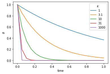
We start with the numerical solution of a very simple differential equation. In fact we choose something simple enough that we already know the answer.
\(\frac{d\theta}{dt} = - k \theta\)
This is the equation which governs radioactive decay, in which case \(\theta\) is the amount of the radioactive isotope remaining and \(d\theta / dt\) is the activity that we can measure. \(k\) is closely related to the half life.
The solution to this equation is
\(\theta(t) = \theta_0 e^{-kt}\)
where \(\theta_0\) is the amount of the radioactive material remaining. The same equation also describes the cooling of, say, a cup of coffee. In this case we interpret \(\theta\) as the excess temperature (above room temperature).
import numpy as npimport matplotlib.pyplot as plt#Set the amount of isotope remaining (i.e. 1=100%)theta_0 =1.0#Create a regularly spaced vector of time values#20 units between 0 and 1.steps=20timelength=1.0time_values = np.linspace(0,timelength,steps)#Try several different values for the half-life, kfor const_k in [1.0, 3.1, 10.0, 31, 100.0]:#This is the solution to the decay equation, how much isotope remains. exact_theta_values = theta_0 * np.exp(-const_k * time_values)#Plot the results for different k values plt.plot(time_values, exact_theta_values)#Add some plot flair plt.legend(('1', '3.1', '10', '31', '1000'),title=r'$k$')plt.xlabel('time')plt.ylabel(r'$\theta$')plt.show()
We want to be able to march forward in time from our starting point (just like the picture above) where \(\theta = \theta_0\) to obtain the value of \(\theta\) at later times. To do this, we need to approximate the original differential equation, and, in particular, the value of the time derivative at each time. There are a number of ways to do this.
First order numerical approximation
Assume that the variation in \(\theta(t)\) is linear, i.e.
\(\theta(t') = \theta_n + \beta t'\)
where we use a local time coordinate \(t' = t - n\Delta t\), so that when we differentiate
\(\frac{d \theta}{dt} = \beta\)
To determine the approximation for the derivative therefore becomes the solution to the following equation:
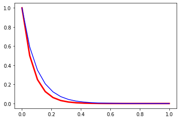
This is a first order difference expression for the derivative which we substitute into the original differential equation for radioactive decay at the current timestep
\(\frac{\theta_{n+1} - \theta_n}{\Delta t} = - k \theta_n\)
This rearranges to give us a time-marching algorithm:
\(\theta_{n+1} = \theta_n (1-k \Delta t)\)
In a moment we will compute some values for this expression to see how accurate it is.
#Set the known constant valuestheta_0 =1.0const_k =10.0#How many timesteps to solvesteps =20timelength =1.0delta_t = timelength / steps#Create a regularly spaced vector of time valuestime_values = np.linspace(0,timelength,steps)#Create an empty array to store the solutionstheta_values = np.zeros(steps)#Set the starting valuestheta_values[0] = theta_0#Step through the time valuesfor i inrange(1, steps):#Find the value for theta at this time step theta_values[i] = theta_values[i-1] * (1- const_k * delta_t)#Compare with the exact solutionexact_theta_values = theta_0 * np.exp(-const_k * time_values)#Plot and compare your resultsplt.plot(time_values, theta_values, linewidth=3.0, color="red")plt.plot(time_values, exact_theta_values, 'b-')
Second Order Runge-Kutta
The Runge-Kutta method can be a more accurate approach to higher order integration solutions. The idea is to estimate the gradient \(d / d t\) at the half way point between two timestep values. This is done in two stages. Initially a first order estimate, \( \) is made for the value of the function \( \) at \(t=t+t /2\) in the future. This value is then subsituted into the differential equation to obtain the estimate for the gradient at this time. The revised gradient is then used to update the original \((t)\) by an entire timestep.
The first order step is \[
\begin{split}
\hat{\theta}(t+\Delta t /2) & = \theta(t) + \left. \frac{d \theta}{d t} \right|_t \frac{\Delta t}{2} \\
&= \theta(t) \left[ 1-\frac{k\Delta t}{2} \right]
\end{split}
\]
Substitute to estimate the gradient at the mid-point \[
\left. \frac{d \theta}{d t} \right|_{t+\Delta t /2} \approx -k \theta(t) \left[ 1-\frac{k\Delta t}{2} \right]
\]
Use this value as the average gradient over the interval \(t\rightarrow t+\Delta t\) to update \(\)
Which gives the Second Order Runge-Kutta estimation for updated \(\theta\) values:
\(\theta(t+\Delta t) \approx \theta(t) \left( 1 - k \Delta t + k^2 \frac{\Delta t^2}{2} \right)\)
Challenge
Can you implement the Second Order Runge-Kutta Numerical Solution in Python? Start as before:
#Set the known constant valuestheta_0 =1.0const_k =10.0#How many timesteps to solvesteps =20timelength =1.0delta_t = timelength / steps#Create a regularly spaced vector of time valuestime_values = np.linspace(0,timelength,steps)#Create an empty array to store the solutionstheta_values = np.zeros(steps)#Set the starting valuestheta_values[0] = theta_0#Step through the time valuesfor i inrange(1, steps):#Find the value for theta at this time step theta_values[????] = ????#Compare with the exact solutionexact_theta_values = theta_0 * np.exp(-const_k * time_values)#Plot and compare your resultsplt.plot(time_values, theta_values, linewidth=3.0, color="red")plt.plot(time_values, exact_theta_values, 'b-')
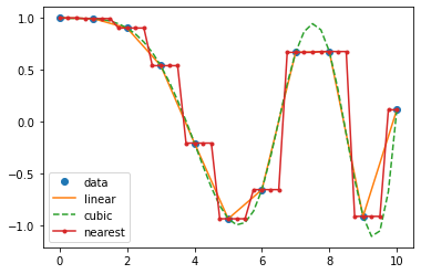
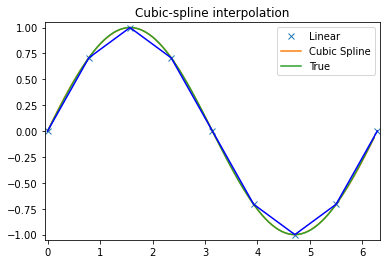
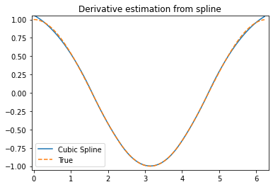
This module provides general interpolation capability for data in 1, 2, and higher dimensions. This list of features is from the documentation:
A class representing an interpolant (interp1d) in 1-D, offering several interpolation methods.
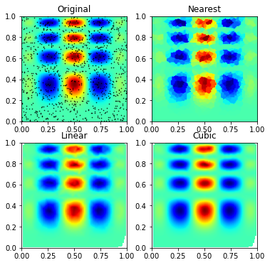
Convenience function griddata offering a simple interface to interpolation in N dimensions (N = 1, 2, 3, 4, …). Object-oriented interface for the underlying routines is also available.
Functions for 1- and 2-dimensional (smoothed) cubic-spline interpolation, based on the FORTRAN library FITPACK. There are both procedural and object-oriented interfaces for the FITPACK library.
Interpolation using Radial Basis Functions.
import matplotlib.pyplot as pltimport numpy as np
1D data
from scipy.interpolate import interp1d
x = np.linspace(0, 10, num=11, endpoint=True)y = np.cos(-x**2/9.0)f = interp1d(x, y, kind='linear') # default if kind=Nonef2 = interp1d(x, y, kind='cubic')f3 = interp1d(x, y, kind='nearest')
There are fewer approaches to n-dimensional data, the evaluation for arbitrary dimensions is always for points on an n dimensional grid.
from scipy.interpolate import griddatadef func(x, y):return x*(1-x)*np.cos(4*np.pi*x) * np.sin(4*np.pi*y**2)**2
# A regular grid array of x,y coordinatesgrid_x, grid_y = np.mgrid[0:1:100j, 0:1:200j] # see np.info(np.mgrid) for an explanation of the 200j !!
np.info(np.mgrid)
`nd_grid` instance which returns a dense multi-dimensional "meshgrid".

An instance of `numpy.lib.index_tricks.nd_grid` which returns an dense
(or fleshed out) mesh-grid when indexed, so that each returned argument
has the same shape.  The dimensions and number of the output arrays are
equal to the number of indexing dimensions.  If the step length is not a
complex number, then the stop is not inclusive.

However, if the step length is a **complex number** (e.g. 5j), then
the integer part of its magnitude is interpreted as specifying the
number of points to create between the start and stop values, where
the stop value **is inclusive**.

Returns
-------
mesh-grid `ndarrays` all of the same dimensions

See Also
--------
lib.index_tricks.nd_grid : class of `ogrid` and `mgrid` objects
ogrid : like mgrid but returns open (not fleshed out) mesh grids
r_ : array concatenator

Examples
--------
>>> np.mgrid[0:5, 0:5]
array([[[0, 0, 0, 0, 0],
        [1, 1, 1, 1, 1],
        [2, 2, 2, 2, 2],
        [3, 3, 3, 3, 3],
        [4, 4, 4, 4, 4]],
       [[0, 1, 2, 3, 4],
        [0, 1, 2, 3, 4],
        [0, 1, 2, 3, 4],
        [0, 1, 2, 3, 4],
        [0, 1, 2, 3, 4]]])
>>> np.mgrid[-1:1:5j]
array([-1. , -0.5,  0. ,  0.5,  1. ])
# A random sampling within the same areapoints = np.random.rand(1000, 2)values = func(points[:,0], points[:,1])# Resample from the values at these points onto the regular meshgrid_z0 = griddata(points, values, (grid_x, grid_y), method='nearest')grid_z1 = griddata(points, values, (grid_x, grid_y), method='linear')grid_z2 = griddata(points, values, (grid_x, grid_y), method='cubic')
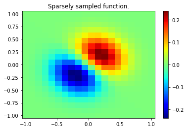
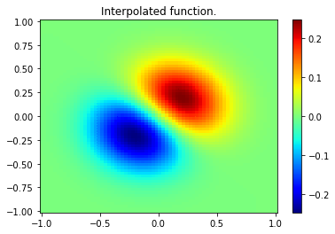
from scipy.interpolate import bisplrep, bisplev# Gridded function (at low resolution ... doesn't need to be gridded data here)x, y = np.mgrid[-1:1:20j, -1:1:20j]z = (x+y) * np.exp(-6.0*(x*x+y*y))plt.figure()plt.pcolor(x, y, z, cmap='jet',shading='auto')plt.colorbar()plt.title("Sparsely sampled function.")plt.show()
xnew, ynew = np.mgrid[-1:1:70j, -1:1:70j]## Create the spline-representation object tcktck = bisplrep(x, y, z, s=0)znew = bisplev(xnew[:,0], ynew[0,:], tck)
Radial basis function interpolation for scattered data in n dimensions (slow for large numbers of points): from scipy.interpolate import Rbf
scipy.ndimage for fast interpolation operations on image-like arrays
B-splines on regular arrays are found in the scipy.signal module
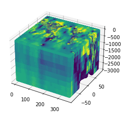
Clustering data with scikit-learn
Here we want to explore a neat and efficient way of exploring a (seisimic tomography) dataset in Python. We will be using a Machine Learning algorithm known as K-Means clustering.
Data is from: Li, C., van der Hilst, R. D., Engdahl, E. R., and Burdick, S. (2008), A new global model for P wave speed variations in Earth’s mantle, Geochem. Geophys. Geosyst., 9, Q05018, doi:10.1029/2007GC001806
from sklearn.cluster import KMeansimport numpy as npimport matplotlib.pyplot as plt from mpl_toolkits.mplot3d import Axes3D
Load in the tomography data set. Assign the column vectors to unique variables (for clarity).
kmeans = KMeans(n_clusters=5, random_state=0).fit(dvp.reshape(-1, 1))#When completed, check the clusters the algorithm has identified.print(kmeans.cluster_centers_)