Table of contents:

1. Brief introduction to profiling, and why we might want to do it

2. Methods to measure function speed/performance

3. Ways to generate function profiles

4. Visualizing and analaysing profiles with call graphs

Why might we need to profile our code

I'm not a computer scientist, let alone a software developer. However, I do work with code and have been envolved with developing software. Sometimes the code that we write is simple and very easy to develop and understand, works perfectly in all situations, and requires little troubleshooting. Unfortunately, that rarely occurs. Profiling can be a useful tool to deploy to help us make our code and software better. Here are a few reasons why.

Long functions can - and will - become hard to understand

Short functions, with few arguments and subroutines, are easy to write, read, and often run very quickly. However, to solve more complex problems we often end up having to use longer functions, or we end up calling upon complex functions within our own functions. As our code increases in length and complexity, it becomes harder for a person to read, and potentially more difficult for a computer to evaluate. This leads directly into the next reason to profile code...

Clear documentation is difficult

Documentation is one of the hardest things to get right, particularly so with long and complex functions or software. Many of the words we use are relatively ambiguous and only make sense within the specific context of our conversations or writing. This can cause problems when writing documentation. Object/variable names and comments may seem clear to the writer, but might not make sense to someone else outside the specific context of the writer's experiences while developing the code.

Something that makes sense to the creator...might make no sense to someone else

And both problems are exacerbated when we collaborate or share our code with others. Something that makes sense to you when you first wrote the code might not make much sense to future you when you are going back to fix a bug 6 months later. It is even less likely to make sense to some other person without your unique perspective and experience if they want to use, adapt, or fix your code in the future.

Profiling can help us address all of these proflems. By profiling our code we can gain a better understanding of what is happening when our code is running. It can help us pinpoint weaknesses and develop better documentation, which will in turn make it easier for our code to be shared with others.

What exactly is profiling?

This quote from the wikipedia article on the subject provides a good summary. While it refers to the use of profiling within classic computer programming settings, all of these reasons to profile can apply to us.

"Program analysis tools are extremely important for understanding program behavior. Computer architects need such tools to evaluate how well programs will perform on new architectures. Software writers need tools to analyze their programs and identify critical sections of code. Compiler writers often use such tools to find out how well their instruction scheduling or branch prediction algorithm is performing..."

"Profiling" actually can refer to several different things:

• "A statistical summary of the events observed", aka profile

• "A stream of recorded events", aka trace

This post will go over several ways to create a statistical summary of events occuring, as well as a record of these events.

A simple example

To start off, here's an example of a very simple function in R. This function takes two arguments. It does some maths with one of the arguments, and it creates two messages based on the two arguments and the result of the maths. Pretty simple stuff, and stuff that R can be very fast at.

MyFirstFunction <- function(x,
                            units
                            ){
  y <- (x*x)*pi

  message("A circle with a radius of ", x, " ", units)
  message("has an area of ", y, " ", units,"^2")
  return(y)
}

MyFirstFunction(42, "cm")

## A circle with a radius of 42 cm

## has an area of 5541.76944093239 cm^2

## [1] 5541.769

But what if you want to know just how fast this function is. How can we measure speed?

How can to measure function speed?

One of the most popular ways to measure function speed is to wrap things in system.time().

system.time(MyFirstFunction(42,"yards"))

##    user  system elapsed 
##   0.001   0.000   0.001

When you run this, you get a measure of the amount of time it took for your function to run. However, this isn't very precise, and it only runs once so you don't get a measure of average speed.

Thankfully, the microbenchmark package provides a lot more functionality. The basic functionality is similar, you wrap your function in microbenchmark() and run it. By default, this will run your function 100 times and record the average time it took to evaluate in microseconds.

library(microbenchmark)
microbenchmark(MyFirstFunction(42,"yards"))

## Unit: microseconds
##                          expr     min       lq     mean   median       uq
##  MyFirstFunction(42, "yards") 276.913 280.5095 291.9876 286.7235 291.5805
##      max neval
##  393.314   100

292 microseconds is pretty darn fast. A simple function like this probably doesn't need to be profiled. But what about a more complex function?

Scenario: complex function, confusing documentation

The reason I started learning about software profiling was because I joined a project to develop an R package that had already started. There were some pretty complex functions with difficult to understand functions. There were also some potential issues with performance. I wanted to scope out performance bottlenecks in the code, and also gain a better understanding of what exactly was going on so I could improve performance.

get_all_images_with_exifs_metadata <- function(images_directory_path,
                                               exifs_attributes_tags_path,
                                               output_path=NULL
)
{
  message("Gathering your images")
  pb <- progress_bar$new(total = 100)
  purrr::walk(1:100, ~{pb$tick(); Sys.sleep(0.1)})
  images_not_having_key_attributes <- c()

  count_of_not_processed_images <- 0

  exifs_tool_path <- Sys.which("exiftool")

  if (is.na(exifs_tool_path) || exifs_tool_path == '') {
    stop("exifs tool not installed. Install ExifTool from https://sno.phy.queensu.ca/~phil/exiftool/ before continue to use this package.",
      "\n")
  }

  # Read user specified attribute tags
  df_exifs_attributes_tags_mapping <- read_csv(exifs_attributes_tags_path, col_names = TRUE, col_types = cols()) %>%
    clean_names()

  # Convert attribute tag mapping to a valid dataframe
  pb <- progress_bar$new(total = 100)
  message("Looking for attribute tags")
  for (i in 1:nrow(df_exifs_attributes_tags_mapping)) {
    pb$tick(0)
    df_exifs_attributes_tags_mapping[i, 2] <- df_exifs_attributes_tags_mapping[i, 2] %>%
      make_clean_names()
  }
  exifs_tagged_attributes <- df_exifs_attributes_tags_mapping[[2]]
  exifs_tagged_attributes <- unlist(strsplit(exifs_tagged_attributes, split=", "))

  message("Processing your images")
  pb <- progress_bar$new(total = 100)
  purrr::walk(1:100, ~{pb$tick(); Sys.sleep(0.1)})
  df <- read_exif(images_directory_path, tags = c("FileName", "CreateDate", "DateTimeOriginal","FileSize", "Keywords"),
    recursive = TRUE, args = NULL, quiet = TRUE)
  # Clean up column names
  df <- df %>%
    separate(FileName, c("File", "Extension"), sep = "[.]") %>%
    mutate(Extension = tolower(Extension))
  df <- df %>%
    clean_names()

  # Filter only the jpg images
  df <- df %>%
    filter(extension == "jpg")

  # Filter only the images which have size greater than 0
  df_valid_images <- df %>%
    filter(file_size > 0)
  df_invalid_images <- df %>%
    filter(file_size == 0)

  # Check if the R data frame has the right keywords
  pb <- progress_bar$new(total = 100)
  purrr::walk(1:100, ~{pb$tick(); Sys.sleep(0.1)})
  message("Checking your data")
  df_valid_images <- get_image_with_exifs_attribute_tag_mapping(df_valid_images, df_exifs_attributes_tags_mapping)
  df_valid_images[df_valid_images == "NA" ] <- NA

  df_valid_images['species'] <- df_valid_images['species_1']
  df_valid_images['count'] <- df_valid_images['no_of_species_1']

  # Creates new rows for each additional species in an image, and converts species names to lower case
  message("Making new rows for additional species")
  df_all_images <- get_additional_species(df_valid_images)
  pb <- progress_bar$new(total = 100)
  purrr::walk(1:100, ~{pb$tick(); Sys.sleep(0.1)})
  df_all_images <- df_all_images %>% mutate(species = tolower(species))

  processed_count <- nrow(df_all_images)
  message("Images successfully wrangled")
  print(processed_count)
  return (df_all_images)
}

What do we want to know about this function?

Here is what I wanted to find out: - What do all of the sub functions do?

• What order are the sub function called in?

• Where are the performance bottlenecks?

• Are any bits of code not being used?

Basic R profiling: Primary data collection tools

Thankfully, R studio has some very powerful built in profiling tools. You can easily use the GUI to interact with these, but you can also interact with them using code.

# Standard built in R profiling tools
library(profvis)
library(proftools)

Basic R profiling: Create a profile of your function

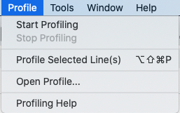
To profile your code, you can just go up to the profiling menu tab and click "start profiling". However, another option is to manually start profiling with code. I've shown how to do this here. I first start profiling with Rprof(), where you can see I specified a name for the profile output to be saved. I then run the code I want to profile. Once this is done, I then stopped profiling byt clicking on the red box in R studio's GUI.

Rprof(filename = "demo_prof.out", # file name for your profile
      append= FALSE,
      interval = 0.02,
      line.profiling = TRUE)
# Run the function you want to profile
test <- get_all_images_with_exifs_metadata(
  "/Users/hlyd4326/Desktop/Some_files",
  "/Users/hlyd4326/Desktop/A_spreadsheet.csv")
# Click on the red box in the console in R studio to end profiling.

Basic R profiling: Results

When you stop profiling, a profile visualization is generated by the profvis package. This visualization shows two things. One shows your code line by line with measurements of memory consumption and time consumption for each line. You also get to see a flame graph, which show long long each bit of code took to run. This can be scrolled and zoomed, but can be a bit hard to understand.

I personally find the line by line measurements to be the most useful bit. Here we can see that two helper functions are consuming a fair chunk of memory and are taking a bit of time to process.

Basic R profiling: Flame Graph

However, you can also bring back in the profile output and manually create a flame graph using a proftools function. This can be more easily read.

pd <- readProfileData("demo_prof.out")
flameGraph(pd)

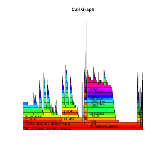
From this flame graph you can see that some portions of the code took the majority of memory/time to run, but also that other portions took a lot of time but really didn't do much. One of those actually ended up being a faulty progress bar that just pointlessly counted down time while nothing was happening.

What did I learn from using R studio's default profiling tools?

• Certain portions of the function accounted for the bulk of memory consumption and compute time.

• The memory utilization did not appear to be optimized: only 12gb of 64gb available RAM were used.

• The inverse of this is that the function should run ok on far less powerful machines.

I still had some questions about how this function was working, so I went to look for more solutions.

What about some sort of call graph?

• Call graphs are a type of control flow diagram, and help us visualise how computer processes function.

• Commonly used in software development to analyse code and improve documentation.

• What tools exist for generating these reports in R?

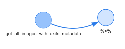
One possibility: visNetwork function dependency graph

I came across a very promising method to makea call graph that used visNetwork's very cool visualizations.

library(DependenciesGraphs)
deps1 <- funDependencies("package:exifpro2camtrapr","get_all_images_with_exifs_metadata")
plot(deps1)

However it doesn't appear to be able to properly understand the pipe opperator. Ironically the documentation for this function wasn't very clear, so I wasn't able to figure out if there was a way to make it so that the function would understand the pipe operator.

Pilgrimage to Bioconductor to find solutions

After much Googling, I found a solution in the documentation of the proftools package: a profile call graph function called plotProfileCallGraph() that would create a nice flow chart of what happens when you run your function.

However, it requires two packages that are not in the CRAN ecosystem. However, they are on Bioconductor

# Here's how to install from Bioconductor:
# install.packages("BiocManager")
# BiocManager::install()

library(graph)
library(Rgraphviz)

Rgraphviz is actually an R implementation of graphviz, which is a very popular tool for making call graphs for many other programming languages.

A call graph that overcomes the pipe

Once I had these packages installed, I could then generate a call graph of my function.

graph1 <- plotProfileCallGraph(pd)

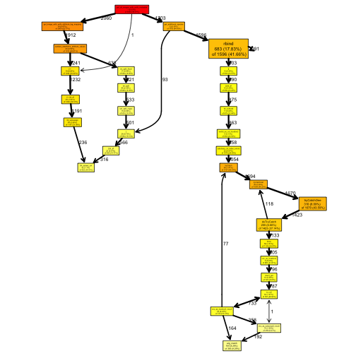
Interestingly, when I generated this while making this post, I realized that I had actually cloned a past development build which had already been optimized somewhat!

A call graph that overcomes the pipe

Here is the call graph I originally created months ago when working on this piece of software. You can see here that there are portions of the function that don't do anything, and that much of the compute time is wasted by the useless progress bars.

How did call graphs help my code?

• They helped me recognize the order in which sub functions and helper functions were called.

• They helped confirm that some portions of code were useless.

However, in the end the code had to be scrapped because of fundamental issues. While profiling and call graphs could help me make sense of the code, the function fundamentally was not built to the proper spec.

Conclusions

• Profiling can help you understand what your code is doing, and when.

• Call graphs can help you visualize complex functions.

• Neither are a substitute for good coding practices.

When I gave this presentation, Joel brought up this famous quote from Donald Knuth: "premature optimization is the root of all evil (or at least most of it) in programming." You probably don't need to worry about profiling every function or measuring the amount of time it takes for a function to calculate the area of a circle. However, when you run into issues or know that your users may likely run into problems, profiling can help us better understand our code. It can help us identify performance bottlenecks and develop better documentation, and in many situations it can help us make our code better.

Bonus: Use Case - HPC

Optimizing code is particularly important when making use of shared HPC resources or using expensive cloud computing resources. However, most of the R profiling techniques I discussed today focused on profiling code that runs locally on individual machines.

When developing R code for use on HPC or other distributed computing, one option is to test code on a local machine and create profiles on code using subsets of data that can run within reasonable time frames on less powerful machines. This way you can identify potential performance bottlenecks locally and hopefully implemement performance improvements before running at full scale on distributed computing.

R packages

# Precise speed metrics
library(microbenchmark) 
# Basic profiling tools
library(profvis)
library(proftools)
# Support for call graphs
library(DependenciesGraphs)
library(graph)
library(Rgraphviz)

         /  /\        ___          /__/\ Thanks
        /  /:/_      /  /\         \  \:\  for
       /  /:/ /\    /  /:/          \__\:\   coming!
      /  /:/ /::\  /__/::\      ___ /  /::\    if
     /__/:/ /:/\:\ \__\/\:\__  /__/\  /:/\:\  you want the slides
     \  \:\/:/~/:/    \  \:\/\ \  \:\/:/__\/   they are going to
      \  \::/ /:/      \__\::/  \  \::/       be on GitHub.
       \__\/ /:/       /__/:/    \  \:\
         /__/:/        \__\/      \  \:\
         \__\/                     \__\/