Getting the dataset
Flight data downloaded from https://raw.githubusercontent.com/apache-superset/examples-data/master/tutorial_flights.csv:
R
library(dplyr)
library(readr)

data <- read_csv("https://raw.githubusercontent.com/apache-superset/examples-data/master/tutorial_flights.csv")
> data %>% glimpse()
Rows: 2,954
Columns: 20
$ Department                <chr> "Orange Department", "Yellow Department", "Yell…
$ Cost                      <dbl> 81.52, 343.98, 25.98, 12.99, 32.97, 61.48, 159.…
$ `Travel Class`            <chr> "Economy", "Economy", "Economy", "Economy", "Ec…
$ `Ticket Single or Return` <chr> "Return", "Return", "Return", "Return", "Return…
$ Airline                   <chr> "Flybe", "Flybe", "Flybe", "Flybe", "Flybe", "F…
$ `Travel Date`             <date> 2011-02-10, 2011-02-11, 2011-03-02, 2011-03-09…
$ `Origin ICAO`             <chr> "EGPF", "EGPF", "EGHI", "EGHI", "EGPE", "EGPE",…
$ `Origin Name`             <chr> "Glasgow International Airport", "Glasgow Inter…
$ `Origin Municipality`     <chr> "Glasgow", "Glasgow", "Southampton", "Southampt…
$ `Origin Region`           <chr> "Scotland", "Scotland", "England", "England", "…
$ `Origin Country`          <chr> "United Kingdom", "United Kingdom", "United Kin…
$ `Origin Latitude`         <dbl> 55.8719, 55.8719, 50.9503, 50.9503, 57.5425, 57…
$ `Origin Longitude`        <dbl> -4.433060, -4.433060, -1.356800, -1.356800, -4.…
$ `Destination ICAO`        <chr> "EGKK", "EGHI", "EGPB", "EPKK", "EGKK", "EGBB",…
$ `Destination Name`        <chr> "London Gatwick Airport", "Southampton Airport"…
$ `Destination Region`      <chr> "England", "England", "Scotland", "Lesser Polan…
$ `Destination Country`     <chr> "United Kingdom", "United Kingdom", "United Kin…
$ `Destination Latitude`    <chr> "51.148102", "50.9502983093262", "59.8788986206…
$ `Destination Longitude`   <chr> "-0.190278", "-1.35679996013641", "-1.295560002…
$ Distance                  <chr> "595", "584", "993", "1493", "753", "584", "508…
Python
import pandas as pd

data = pd.read_csv("https://raw.githubusercontent.com/apache-superset/examples-data/master/tutorial_flights.csv")
>>> data.columns
Index(['Department', 'Cost', 'Travel Class', 'Ticket Single or Return',
       'Airline', 'Travel Date', 'Origin ICAO', 'Origin Name',
       'Origin Municipality', 'Origin Region', 'Origin Country',
       'Origin Latitude', 'Origin Longitude', 'Destination ICAO',
       'Destination Name', 'Destination Region', 'Destination Country',
       'Destination Latitude', 'Destination Longitude', 'Distance'],
      dtype='object')
Creating New columns from old ones
R
> data %>%
  group_by(`Destination Country`) %>%
  mutate(
    total_cost_per_country = sum(Cost),
    tot_cost_country_euro = total_cost_per_country * 1.3
  ) %>%
  glimpse()
Rows: 2,954
Columns: 22
Groups: Destination Country [65]
$ Department                <chr> "Orange Department", "Yellow Department", "Yello…
$ Cost                      <dbl> 81.52, 343.98, 25.98, 12.99, 32.97, 61.48, 159.8…
$ `Travel Class`            <chr> "Economy", "Economy", "Economy", "Economy", "Eco…
$ `Ticket Single or Return` <chr> "Return", "Return", "Return", "Return", "Return"…
$ Airline                   <chr> "Flybe", "Flybe", "Flybe", "Flybe", "Flybe", "Fl…
$ `Travel Date`             <date> 2011-02-10, 2011-02-11, 2011-03-02, 2011-03-09,…
$ `Origin ICAO`             <chr> "EGPF", "EGPF", "EGHI", "EGHI", "EGPE", "EGPE", …
$ `Origin Name`             <chr> "Glasgow International Airport", "Glasgow Intern…
$ `Origin Municipality`     <chr> "Glasgow", "Glasgow", "Southampton", "Southampto…
$ `Origin Region`           <chr> "Scotland", "Scotland", "England", "England", "S…
$ `Origin Country`          <chr> "United Kingdom", "United Kingdom", "United King…
$ `Origin Latitude`         <dbl> 55.8719, 55.8719, 50.9503, 50.9503, 57.5425, 57.…
$ `Origin Longitude`        <dbl> -4.433060, -4.433060, -1.356800, -1.356800, -4.0…
$ `Destination ICAO`        <chr> "EGKK", "EGHI", "EGPB", "EPKK", "EGKK", "EGBB", …
$ `Destination Name`        <chr> "London Gatwick Airport", "Southampton Airport",…
$ `Destination Region`      <chr> "England", "England", "Scotland", "Lesser Poland…
$ `Destination Country`     <chr> "United Kingdom", "United Kingdom", "United King…
$ `Destination Latitude`    <chr> "51.148102", "50.9502983093262", "59.87889862060…
$ `Destination Longitude`   <chr> "-0.190278", "-1.35679996013641", "-1.2955600023…
$ Distance                  <chr> "595", "584", "993", "1493", "753", "584", "508"…
$ total_cost_per_country    <dbl> 376846.33, 376846.33, 376846.33, 4968.51, 376846…
$ tot_cost_country_euro     <dbl> 489900.229, 489900.229, 489900.229, 6459.063, 48…
Python
Same as above, and printing out the first 5 rows of the last 5 columns:
(
    data.assign(
        total_cost_per_country=lambda x: (
            x[["Destination Country", "Cost"]].groupby("Destination Country")["Cost"]
            .transform("sum")
        ),
        tot_cost_country_euro=lambda x: x["total_cost_per_country"] * 1.3
    )
    .iloc[:5, -5:]
    .to_markdown()
)
Code output:
| Destination Latitude | Destination Longitude | Distance | total_cost_per_country | tot_cost_country_euro | |
|---|---|---|---|---|---|
| 0 | 51.1481 | -0.190278 | 595 | 376846.33 | 489900.23 |
| 1 | 50.9503 | -1.3568 | 584 | 376846.33 | 489900.23 |
| 2 | 59.8789 | -1.29556 | 993 | 376846.33 | 489900.23 |
| 3 | 50.0777 | 19.7848 | 1493 | 4968.51 | 6459.06 |
| 4 | 51.1481 | -0.190278 | 753 | 376846.33 | 489900.23 |
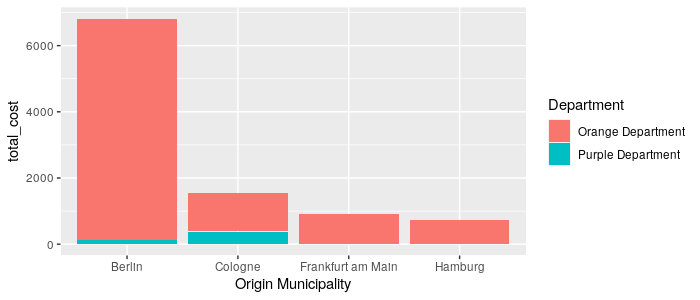
Data viz example
A classic groupby, apply aggregation and filtering and plot stuffs
R
data %>%
  filter(`Origin Country` == "Germany") %>%
  # glimpse()
  select(`Origin Municipality`, Cost, Department) %>%
  group_by(`Origin Municipality`) %>%
  mutate(total_cost = sum(Cost)) %>%
  ggplot(data = ., mapping = aes(x = `Origin Municipality`, y = total_cost, fill = Department)) +
  geom_bar(stat = "identity")
Output:
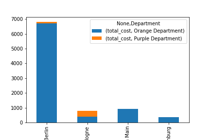
Python
(
    data[data["Origin Country"] == "Germany"]
    .groupby(["Origin Municipality", "Department"])
    .agg(
        total_cost=pd.NamedAgg(column="Cost", aggfunc="sum"),
    )
    .reset_index()
    .pivot_table(
        index=["Origin Municipality"],
        columns=["Department"],
        values=["total_cost"]
    )
    .plot.bar(stacked=True)
    .get_figure()
)
Output:
Data pipelines
A classic data pipeline with loading, processing, writing steps:
R
read_data <- function(filename) {
  df  <- read_csv(filename, ...)
  return(df)
}

process_data <- function(df) {
  df_out <- df %>%
    group_by("group_col") %>%
    mutate(
      new_col1 = max(col1),
      new_col2 = sum(col2)
    )
  ...
  return(df_out)
}

write_data <- function(df, outfilename) {
  df_out <- df %>%
    select(-col1, -col2)
  write_csv(df_out, outfilename)

  return(df_out)
}
data <- read_data(filename = "path/to/input/file") %>%
  process_data(df = .) %>%
  write_data(df = ., outfilename = "path/to/output/file")
Python
def read_data(filename: str) -> Dataframe:
    df = pd.read_csv(filename, colums = , ...)
    return df

def process_data(df: Dataframe):
    df_out = df
    df_out[["new_col1", "new_col2"]] = (
        df[["group_col", "col1", "col2"]].groupby("group_col")
        .agg({
            "col1": "max",
            "col2": "sum",
        })
    )
    ...
    return df_out

def write_data(df: Dataframe, outfilename):
    df_out = df.drop(["col1", "col2"], axis=1)
    df_out.write(outfilename)
    return df_out
data = (
    read_data("path/to/input/file")
    .pipe(process_data)
    .pipe(write_data, outfilename="path/to/output/file")
)