Introduction

Overview

recocam provides robust tools for extracting and processing information and annotations that have been stored in image EXIF data. This package was built to support ecologists who have to deal with large numbers of images from camera traps and to prepare them for analysis with the camtrapr package, but it can work with all sorts of images as long as they contain annotation that have been stored in the keywords EXIF attribute field. This package was developed by the Sydney Informatics Hub, a Core Research Facility of the University of Sydney.

This package is designed to be computationally efficient and can process multiple subfolders full of images, but be aware that processing time goes up as more images are included. Current processing speed for the main importing function gather_images() is around 100 images a second.

This package allows users to generate a data frame of information contained in image EXIF data, and can adapt to different tagging schemes as long as they follow a structure (see below). The other functions in the package are designed to enable users to use their image data with camtrapr’s data exploration tools.

Installation

Before you can install and use exifpro2xamtrapr, you must install one program (ExifTool, a free and open source program for extracting image metadata) and a few R packages (notably exifr to enable efficient use of ExifTool, with reshape2 and Tidyverse providing some important code functionality).

ExifTool

The method for installing ExifTool on your computer varies depending on if you are using MacOS/Linux/Unix or Windows. You can find out more about ExifTool and download the software here.

On MacOS/Linux/Unix, simply follow the steps provided on ExifTool’s website. For Windows, you will have take a couple extra steps to ensure that R is able to utilize ExifTool. Once you have downloaded the stand-alone executable, unzip the file and rename the .exe file to “exiftool.exe”. Then place this file in your primary windows directory (C:/Windows in most cases). Once you have done this, R should be able to find ExifTool.

To make sure that you have correctly installed ExifTool:

#Check if your system is able to find ExifTool
Sys.which("exiftool")

##                  exiftool 
## "/usr/local/bin/exiftool"

#This is what you would see on MacOS. On Windows, you should see "C:\\WINDOWS\\exiftool.exe"

recocam

To install recocam, you can download it from the Sydney Informatics Hub’s github.

#something like this, placeholder now
library(devtools)
install_github("https://github.com/Sydney-Informatics-Hub/recocam")

If you have any questions about this package, run into any issues, or simply want to see what is going on with development of recocam, check out the repository’s issues page here.

Citing recocam

If you use recocam for a publication, presentation, or any form professional application, please cite recocam as well as the Sydney Informatics Hub, a Core Research Facility of the University of Sydney.

Using recocam

library(recocam)
library(tidyverse) # this should automatically load, but just in case it doesn't here is the command

## ── Attaching packages ──────────────────────────────────────────────────────────────────────────────────────────────────────────── tidyverse 1.3.0 ──

## ✓ ggplot2 3.3.0     ✓ purrr   0.3.4
## ✓ tibble  3.0.1     ✓ dplyr   0.8.5
## ✓ tidyr   1.0.2     ✓ stringr 1.4.0
## ✓ readr   1.3.1     ✓ forcats 0.5.0

## ── Conflicts ─────────────────────────────────────────────────────────────────────────────────────────────────────────────── tidyverse_conflicts() ──
## x dplyr::filter() masks stats::filter()
## x dplyr::lag()    masks stats::lag()

Workflow

The workflow for recocam has three main steps. Each of these steps involves its own unique functions that together greatly simplify the process of dealing with camera trap images.

Extracting and transforming raw data
- Reading information from image exif data
- Mapping image exif data to your tagging scheme
Transforming your data into a form that can be used with camtrapr
Creating a recordsTable with rows for each observation
Creating a ctTable with information about camera trap efforts

Data preperation

This package assumes that you have a set of camera trap photos that have been tagged with information about the camera, trip, species sighted, etc. This sort of tagging is usually done manually either through a program like ExifPro or some other way of adding information to image files.

Before you start, you will want to have three things prepared in advance. First, is the path to the images that you want to analyse. You can find this by right/command clicking on the folder and clicking “properties” or “get info” respectively if you are using Windows or MacOS.

Second, you will need to provide a csv file with information that will be used to label the tags within the keywords exif attribute of your images. Your csv file must have two columns: the first containing the number of each tag (the “Index”), and the second with a label for what each tag is representing (the “ExifAttribute”). Here is an example, from the tagging scheme used by the Desert Ecology Research Group at the University of Sydney:

## # A tibble: 6 x 2
##   Index ExifAttribute   
##   <dbl> <chr>           
## 1     1 Trip            
## 2     2 Site            
## 3     3 Treatment       
## 4     4 Camera no.      
## 5     5 Species 1       
## 6     6 no. of species 1

Finally, you will need to provide a csv file containing information about your camera trap locations. In this example (also from DERG), there are geographic (latitude and longitude) coordinates for each camera location. For the purposes of this vignette, we have replaced the actual coordinates with some random points chosen near Concordia Station in Antarctica to protect the locations of any endangered and protected species.

## # A tibble: 6 x 6
##   SiteCode   lat  long Site              Camera_Tra Notes         
##   <chr>    <dbl> <dbl> <chr>             <chr>      <chr>         
## 1 CamMC3   -68.6  135. Main Camp North   Camera R10 Reconynx PC800
## 2 CamMC4   -68    134. Main Camp North   Camera R27 Reconynx PC800
## 3 CamMC2   -68.2  133. Main Camp South   Camera R12 Reconynx PC800
## 4 CamMC1   -68.0  136. Main Camp South   Camera R03 Reconynx PC800
## 5 CamFRS1  -68.6  135. Field River South Camera R16 Reconynx PC800
## 6 CamFRS2  -68.2  135. Field River South Camera R19 Reconynx PC800

Importing data with gather_images

The gather_images function extracts information contained in the EXIF data of your images and transforms that information into something much more easily usable for further analysis, using your keywords spreadsheet to help correctly interpret the information in the exif attributes of each image.

That also means that this function is the most computationally complex in this package. For example, it takes approximately one minute to process 10,000 images that are stored on a solid state hard drive; it takes far longer to process images that are stored on a remote server. We recommend that you transfer images onto your hard drive when using this function.

image_folder <- system.file("extdata/testimages", package="recocam")
keywords <- system.file("testdata/keywords.csv", package="recocam")

test_raw <- gather_images(image_folder, keywords)

glimpse(test_raw)

## Rows: 30
## Columns: 16
## $ trip               <chr> "Apr.14", "Apr.14", "Apr.14", "Apr.14", "Apr.14", …
## $ site               <chr> "Norries Bore", "Norries Bore", "Norries Bore", "N…
## $ treatment          <chr> "Fox and goanna removal", "Fox and goanna removal"…
## $ camera_no          <chr> "R17", "R17", "R17", "R17", "R17", "R17", "R17", "…
## $ species_1          <chr> "cat", NA, NA, NA, NA, NA, NA, NA, NA, "cat", NA, …
## $ no_of_species_1    <chr> "1", NA, NA, NA, NA, NA, NA, NA, NA, "1", NA, NA, …
## $ species_2          <chr> NA, NA, NA, NA, NA, NA, NA, NA, NA, NA, NA, NA, NA…
## $ no_of_species_2    <chr> NA, NA, NA, NA, NA, NA, NA, NA, NA, NA, NA, NA, NA…
## $ comments           <chr> NA, NA, NA, NA, NA, NA, NA, NA, "first photo taken…
## $ moon_phase_number  <chr> "2", NA, NA, NA, NA, NA, NA, NA, NA, "2", NA, NA, …
## $ site_code          <chr> "CamNB2", "CamNB2", "CamNB2", "CamNB2", "CamNB2", …
## $ source_file        <chr> "/private/var/folders/0s/scmv3h_12_b66n4w_0rn4qrh0…
## $ file_name          <chr> "NBR172014-04_0013.jpg", "NBR172014-04_0007.jpg", …
## $ date_time_original <chr> "2013:10:09 17:55:13", "2013:10:01 22:00:54", "201…
## $ file_size          <chr> "533135", "277693", "474973", "351488", "461175", …
## $ process_image      <chr> "TRUE", "TRUE", "TRUE", "TRUE", "TRUE", "TRUE", "T…

You can now see that there is a large tibble containing all of the information that was extracted from your images.

If you want to analyse your data with camtrapr, you next will need to use the prep_camtrapr() function to process perform some transformations on the data. This function makes one big assumption: that you have tagged your images following this scheme: individual species in images identified by “species_1”, “species_2”, etc. and counts of each species identified by “no_of_species_1” etc. This function will work with any number of possible species in an image, but by default it will look for two species.

season1_raw <- readRDS(system.file("extdata/vignette_raw1.Rds", package="recocam"))

season1_clean <- prep_camtrapr(season1_raw, number_of_species = 2)

Creating a recordsTable

The first data frame that we want to create is what camtrapR calls a “recordsTable”. This function is adapted from their package, and will create a recordsTable based on the data we just extracted from your images.

season1_records <- make_recordtable(season1_clean)

Creating a ctTable

Finally, you can use a file containing informations about your camera trap locations to create a data frame with information about camera efforts, also known as a “ctTable”, for analysis in camtrapR. Note that you need to specify the “trip”: this is the particular trapping season or period you are analysing and it should be written as a three letter month and abbreviated year seperated with a period. For example: if you are analyzing images from June 2010, you would abbreviate this as “Jun.10”.

camsites <- system.file("extdata/CamSitesDemo.csv", package="recocam")

season1_efforts <- make_effortstable(season1_clean, camsites, trip = "Jun.10")

Working with multiple data sets

If you’d like to combine information from multiple seasons together, you can merge these tables in several different ways using functions from the dplyr package.

First, lets load in some files from another fieldwork season.

season2_clean <- readRDS(system.file("/extdata/vignette_clean2.Rds", package= "recocam"))
season2_records <- readRDS(system.file("/extdata/vignette_records2.Rds", package= "recocam"))
season2_efforts <- readRDS(system.file("/extdata/vignette_efforts2.Rds", package= "recocam"))

Next, we will simply join these files with the ones from the season that we just processed.

merged_images_clean <- dplyr::bind_rows(season1_clean, season2_clean)
merged_records <- dplyr::bind_rows(season1_records, season2_records)
merged_efforts <- dplyr::bind_rows(season1_efforts, season2_efforts)

You can now perform operations on these as normal.

Example analysis with camtrapR

library(camtrapR)
library(rgdal)

You can now take the two output data frames and use them for a wide variety of analyses with camtrapR. Here are examples, based on camtrapR’s data exploration vignette.

Activity density analysis

Activity density plots can be easily generated using camtrapR. One important thing to note is that there are many different arguments for the “activityDensity” function, and it is very important to make sure that you specify the names of the particular columns that your data is coming from.

activityDensity(recordTable = season1_records,
                allSpecies = TRUE,
                speciesCol = "species",
                recordDateTimeCol = "date_time_original"
                )

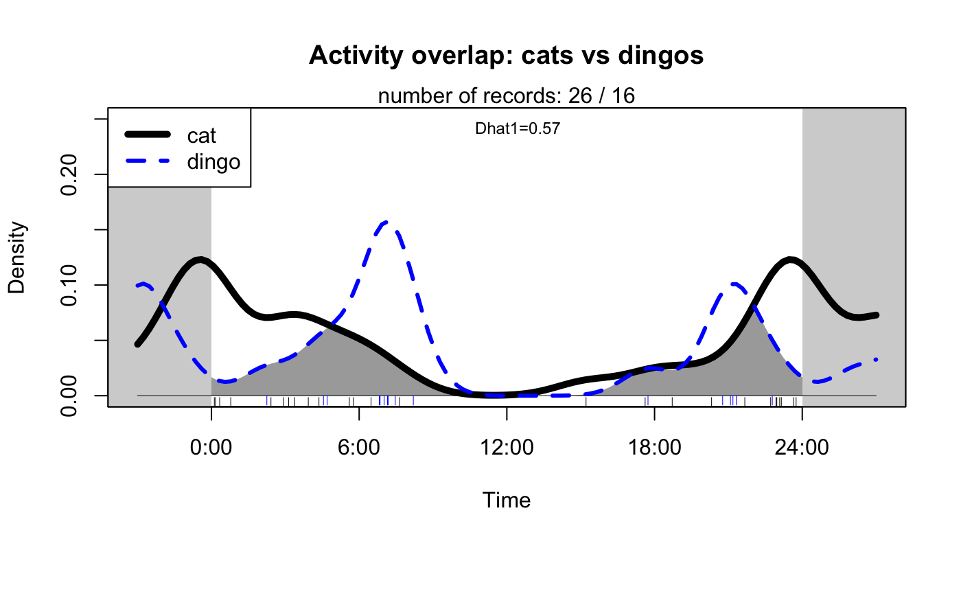
One particularly useful feature of camtrapR is the ability to plot the activity of two different species at the same time. For example, here the activity of two potentially competing predators is plotted. These observations can provide very useful insights about how different species may or may not be interacting, or utilizing different times of the day.

activityOverlap(recordTable = season1_records,
                speciesA = "cat",
                speciesB = "dingo",
                speciesCol = "species",
                recordDateTimeCol = "date_time_original",
                writePNG    = FALSE,
                plotR       = TRUE,
                createDir   = FALSE,
                pngMaxPix   = 1000,
                linecol     = c("black", "blue"),
                linewidth   = c(5,3),
                linetype    = c(1, 2),
                olapcol     = "darkgrey",
                add.rug     = TRUE,
                extend      = "lightgrey",
                ylim        = c(0, 0.25),
                main        = paste("Activity overlap: cats vs dingos")
)

Spatial Analysis

Richness and Abundance

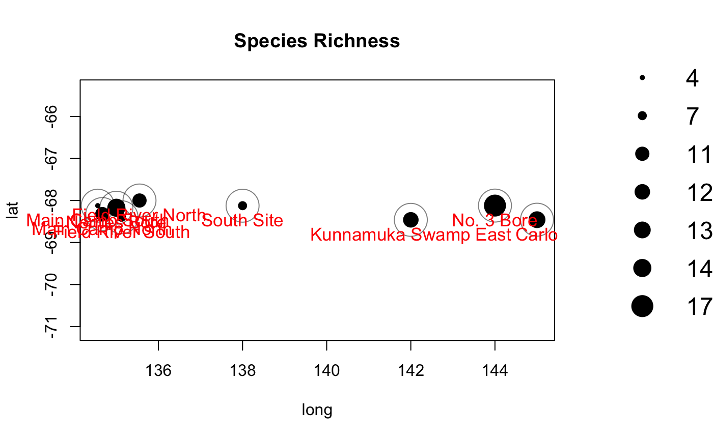
You can easily plot species richness observed at each of your cameras.

maptest1 <- detectionMaps(CTtable = season1_efforts,
                          recordTable = season1_records,
                          Xcol = "long",
                          Ycol = "lat",
                          stationCol = "site",
                          speciesCol = "species",
                          printLabels  = TRUE,
                          richnessPlot = TRUE,
                          speciesPlots = FALSE,
                          addLegend    = TRUE
)

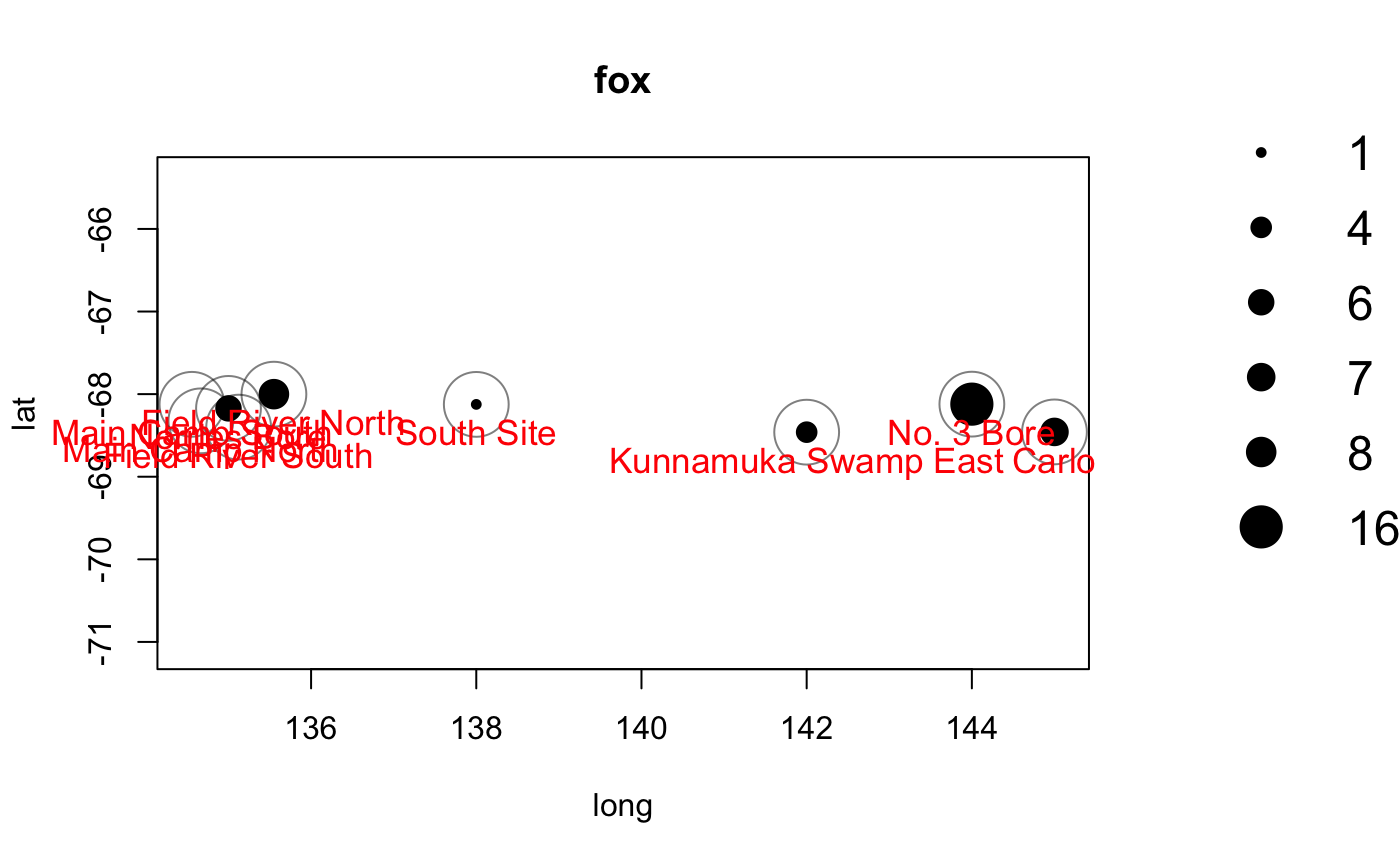
Or you can plot abundance of individual species.

season1_cats <- season1_records[season1_records$species == "cat",]

season1_catmap <- detectionMaps(CTtable      = season1_efforts,
                           recordTable   = season1_cats,
                           Xcol = "long",
                           Ycol = "lat",
                           stationCol = "site",
                           speciesCol = "species",
                           printLabels  = TRUE,
                           richnessPlot = FALSE,
                           speciesPlots = TRUE,
                           addLegend    = TRUE
)

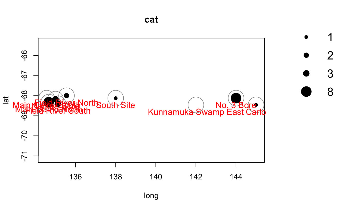
You can then make observations about the differing distributions and ranges of different species in your study area.

Shapefiles

You can also export shapefiles of your data. Shapefiles can be used to perform powerful spatial analysis or create easily understandably and engaging maps.

shapefileName <- "VignetteShp"
shapefileProjection <- "+init=epsg:4326"

Mapstest3 <- detectionMaps(CTtable = season1_efforts,
                           recordTable = season1_records,
                           Xcol = "long",
                           Ycol = "lat",
                           stationCol = "site",
                           speciesCol = "species",
                           richnessPlot        = FALSE,         # no richness plot
                           speciesPlots        = FALSE,         # no species plots
                           writeShapefile      = TRUE,          # but shaepfile creation
                           shapefileName       = shapefileName,
                           shapefileDirectory  = tempdir(),
                           shapefileProjection = shapefileProjection
)

Lets check if that shapefile works! Alternatively, you can also open this shapefile in your preferred GIS programme.

season1_shapefile <- readOGR(dsn   = tempdir(),
                         layer = "VignetteShp")

season1_shapefile@data

detections_spdf <- SpatialPointsDataFrame(coords      = Mapstest3[,c("lat", "long")],
                                          data        = Mapstest3,
                                          proj4string = CRS(shapefileProjection))

str(detections_spdf)

Example with leaflet

While camtrapR contains some useful tools for plotting maps, you can now take this data and plot maps using popular packages such as ggplot2 and leaflet. Both of these provide very powerful options for visualizing your data and creating publication ready graphics.

In this quick example, I’ll show you how you can use leaflet to visualize the shapefile exported by camtrapR.

First, we will load in the required packages and bring the shapefile back in to R.

library(sf)

## Linking to GEOS 3.7.2, GDAL 2.4.2, PROJ 5.2.0

library(sp)
season1_shapefile <- system.file("/extdata/VignetteShp.shp", package = "recocam")

cam_shp <- readOGR(season1_shapefile)

## OGR data source with driver: ESRI Shapefile 
## Source: "/private/var/folders/0s/scmv3h_12_b66n4w_0rn4qrh0000gp/T/Rtmpb1Gg5J/temp_libpath3ada56659b07/recocam/extdata/VignetteShp.shp", layer: "VignetteShp"
## with 9 features
## It has 38 fields

cam_shp <- spTransform(cam_shp, CRS("+init=epsg:4326"))

Next, lets plot it with leaflet.

library(leaflet)
library(leaflet.extras)
library(leaflet.providers)
# define a palette based on our shapefile
pal <- colorNumeric(
  palette = "Spectral",
  domain = cam_shp$n_specs
)

cam_shp %>% leaflet() %>%
  addProviderTiles(providers$Stamen.Terrain,
                   options = providerTileOptions(noWrap = TRUE),
                   group = "Map") %>%
  addProviderTiles(providers$Esri.WorldImagery,
                   options = providerTileOptions(noWrap = TRUE),
                   group = "Satellite")  %>%
  addCircleMarkers(stroke = FALSE,
                   fillOpacity = 1,
                   radius = ~n_specs,
                   color= ~pal(cam_shp$n_specs),
                   label = ~site
                   ) %>%
  addLayersControl(baseGroups = c("Map", "Satellite")) %>%
  addLegend(position = "topright",
            pal = pal,
            values = cam_shp$n_specs,
            title = "Species Richness",
            opacity = 1,
            group = "Richness") %>%
  addScaleBar(position="bottomleft") %>%
  addMiniMap()

Bonus Tips and Tricks

Removing columns from data

What if you decide to merge two data frames of data extracted from images using gather_images(), and R gives you an error message telling you that it cannot merge these two data frames because there are different numbers of columns? Don’t panic! This situation could be caused by a couple different things, and it is pretty easy to work around it.

head(test_raw)

## # A tibble: 6 x 16
##   trip  site  treatment camera_no species_1 no_of_species_1 species_2
##   <chr> <chr> <chr>     <chr>     <chr>     <chr>           <chr>    
## 1 Apr.… Norr… Fox and … R17       cat       1               <NA>     
## 2 Apr.… Norr… Fox and … R17       <NA>      <NA>            <NA>     
## 3 Apr.… Norr… Fox and … R17       <NA>      <NA>            <NA>     
## 4 Apr.… Norr… Fox and … R17       <NA>      <NA>            <NA>     
## 5 Apr.… Norr… Fox and … R17       <NA>      <NA>            <NA>     
## 6 Apr.… Norr… Fox and … R17       <NA>      <NA>            <NA>     
## # … with 9 more variables: no_of_species_2 <chr>, comments <chr>,
## #   moon_phase_number <chr>, site_code <chr>, source_file <chr>,
## #   file_name <chr>, date_time_original <chr>, file_size <chr>,
## #   process_image <chr>

glimpse(test_raw)

## Rows: 30
## Columns: 16
## $ trip               <chr> "Apr.14", "Apr.14", "Apr.14", "Apr.14", "Apr.14", …
## $ site               <chr> "Norries Bore", "Norries Bore", "Norries Bore", "N…
## $ treatment          <chr> "Fox and goanna removal", "Fox and goanna removal"…
## $ camera_no          <chr> "R17", "R17", "R17", "R17", "R17", "R17", "R17", "…
## $ species_1          <chr> "cat", NA, NA, NA, NA, NA, NA, NA, NA, "cat", NA, …
## $ no_of_species_1    <chr> "1", NA, NA, NA, NA, NA, NA, NA, NA, "1", NA, NA, …
## $ species_2          <chr> NA, NA, NA, NA, NA, NA, NA, NA, NA, NA, NA, NA, NA…
## $ no_of_species_2    <chr> NA, NA, NA, NA, NA, NA, NA, NA, NA, NA, NA, NA, NA…
## $ comments           <chr> NA, NA, NA, NA, NA, NA, NA, NA, "first photo taken…
## $ moon_phase_number  <chr> "2", NA, NA, NA, NA, NA, NA, NA, NA, "2", NA, NA, …
## $ site_code          <chr> "CamNB2", "CamNB2", "CamNB2", "CamNB2", "CamNB2", …
## $ source_file        <chr> "/private/var/folders/0s/scmv3h_12_b66n4w_0rn4qrh0…
## $ file_name          <chr> "NBR172014-04_0013.jpg", "NBR172014-04_0007.jpg", …
## $ date_time_original <chr> "2013:10:09 17:55:13", "2013:10:01 22:00:54", "201…
## $ file_size          <chr> "533135", "277693", "474973", "351488", "461175", …
## $ process_image      <chr> "TRUE", "TRUE", "TRUE", "TRUE", "TRUE", "TRUE", "T…

To start, diagnose why there are different numbers of columns. Data exploration functions like head() and tibble::glimpse() can be very useful for this. Use these to see what columns each of your data frames share, and which ones they don’t. To merge them together easily, you want to make sure that both data frames have exactly the same columns.

So, from head() and glimpse() we know that are data frame has 16 columns. But what if we want to merge it with one that has 15 columns, and we’ve identified that the data frame we want to merge with does not have a “comments” column? We can deal with this very easily using dplyr::select().

test_raw2 <- test_raw %>%
  dplyr::select(!comments) # by writing "!comments", we are actually selecting all columns except for comments

test_raw2

## # A tibble: 30 x 15
##    trip  site  treatment camera_no species_1 no_of_species_1 species_2
##    <chr> <chr> <chr>     <chr>     <chr>     <chr>           <chr>    
##  1 Apr.… Norr… Fox and … R17       cat       1               <NA>     
##  2 Apr.… Norr… Fox and … R17       <NA>      <NA>            <NA>     
##  3 Apr.… Norr… Fox and … R17       <NA>      <NA>            <NA>     
##  4 Apr.… Norr… Fox and … R17       <NA>      <NA>            <NA>     
##  5 Apr.… Norr… Fox and … R17       <NA>      <NA>            <NA>     
##  6 Apr.… Norr… Fox and … R17       <NA>      <NA>            <NA>     
##  7 Apr.… Norr… Fox and … R17       <NA>      <NA>            <NA>     
##  8 Apr.… Norr… Fox and … R17       <NA>      <NA>            <NA>     
##  9 Apr.… Norr… Fox and … R17       <NA>      <NA>            <NA>     
## 10 Apr.… Norr… Fox and … R17       cat       1               <NA>     
## # … with 20 more rows, and 8 more variables: no_of_species_2 <chr>,
## #   moon_phase_number <chr>, site_code <chr>, source_file <chr>,
## #   file_name <chr>, date_time_original <chr>, file_size <chr>,
## #   process_image <chr>

You can now see that we have removed the comments column. Now to merge this data frame with that hypothetical comments-less data frame, you can use dplyr::bind_rows()

Wrangling camera trap images with recocam

Henry Lydecker

2020-05-04