2.3.1 Generalisability: who and what the findings apply to

Learning objectives

Use the metadata recorded about an example cohort to state who a study's findings do and do not apply to
Evaluate the trade-off between narrowing a cohort for power and broadening it for generalisability
Apply those trade-offs to recommend a follow-up design or a reallocation of resources between depth and coverage

The two previous sections of Module 2 asked whether the measurements were trustworthy and whether there were enough of them to detect an effect. This section asks a third question: who and what does the finding apply to?

Generalisability describes how far a study's findings extend beyond the specific samples and conditions in which they were produced. Every study is conducted on a defined group like particular individuals, a particular tissue, under particular conditions, at a particular time. The measurements describe that group. Whether they also describe other groups, other tissues, or other conditions is the generalisability question.

Generalisability is sometimes called external validity, meaning how well the findings hold outside the study. This is different from internal validity, which asks whether the comparison within the study is trustworthy. In other words, did the observed difference between groups reflect real world biological patterns or some internal factor? A study can have strong internal validity and still have narrow generalisability. These are different questions and they are addressed by different parts of the design.

The narrower a study's scope, the more precisely a interpretation can be made, but can make external comparisons difficult. This is not a flaw. A study designed and reported with clear limits is more useful than one that overclaims. The problem is not scope; it is claiming past the design.

Components of generalisability

Before asking how generalisable a finding is, it helps to be precise about what generalising means. There are two distinct components:

Population generalisability: which samples or organisms the finding applies to. This is determined by the study population: what was sampled, from which settings, and at which stage of the biological process or disease.
Biological scope: what the finding covers. This is determined by the platform and sampling strategy: which molecular layer was measured, in which tissue or sample type, and at which time point. A transcriptomic finding from liver tissue does not describe what is happening in kidney.

Activity: where does the conclusion exceed the design?

Each scenario below describes a study and a conclusion drawn from it. For each one:

Identify a population generalisability failure: who does the study actually describe, and who is the conclusion wrongly extended to?
Identify a biological scope failure: what does the measurement actually capture, and what is the conclusion wrongly claiming it covers?

Choose the scenario most relevant to your field, or work through all five.

Scenario 1: Genome

A GWAS of 480,000 individuals of European ancestry identifies 34 variants associated with type 2 diabetes risk. The authors conclude: "These variants can be used to calculate polygenic risk scores to identify individuals at elevated risk of type 2 diabetes."

Answers

Population: The cohort is European-ancestry only. Allele frequencies and linkage disequilibrium patterns differ between populations; polygenic risk scores built from European GWAS are substantially less accurate in people of other ancestries. The conclusion claims a general risk tool; the design produced one that works primarily in European-ancestry individuals.

Scope: Identifying associated variants does not establish what those variants do biologically or in which tissue they act. A variant in a regulatory region may influence gene expression only in a specific cell type like pancreatic beta cells, adipocytes, or liver hepatocytes, that was never measured. The GWAS identifies statistical associations; the molecular mechanism and tissue of action require further experiments.

Scenario 2: Epigenome

ATAC-seq is performed on CD4+ T cells isolated from peripheral blood of 30 patients with active rheumatoid arthritis and 30 healthy controls. The authors report 1,240 differentially accessible chromatin regions and conclude: "These regulatory elements control the gene expression changes that drive rheumatoid arthritis pathology."

Answers

Population: The study uses CD4+ T cells from peripheral blood of patients with active disease. Whether the same chromatin changes are present in other immune cell types, in patients with early or remitting disease, or in other populations is not established.

Scope: Chromatin state is established separately in each cell type. The accessible regions in circulating CD4+ T cells do not describe the regulatory state in synovial fibroblasts, tissue-resident macrophages, or other cell types at the site of joint inflammation — where much of RA pathology is driven. Blood is not a proxy for the epigenome of joint tissue.

Scenario 3: Transcriptome

Bulk RNA-seq is performed on liver tissue from male C57BL/6 mice fed a high-fat diet for 12 weeks versus standard chow controls. The authors report upregulation of lipid metabolism and inflammatory pathways and conclude: "High-fat diet induces a conserved transcriptional programme in the liver that drives metabolic dysfunction."

Answers

Population: The study uses one inbred mouse strain (C57BL/6), one sex (male), one diet duration (12 weeks), and one age. Transcriptional responses to high-fat diet differ between strains and sexes. "Conserved" implies generality across species and conditions; the design tests one narrow configuration.

Scope: Bulk liver RNA-seq averages expression across all liver cell types — hepatocytes, Kupffer cells, stellate cells, endothelial cells. An upregulated lipid metabolism gene could reflect increased activity in hepatocytes, an expansion of a cell population that already expresses that gene at high levels, or both. The data cannot attribute the change to a specific cell type or process without single-cell or sorted-population data.

Scenario 4: Proteome

Plasma proteomics is performed on 45 individuals with early Alzheimer's disease and 45 age-matched cognitively normal controls. The authors identify 18 proteins at significantly different concentrations and conclude: "These proteins are biomarkers of Alzheimer's disease pathology and reflect the molecular changes occurring in the brain."

Answers

Population: The study is restricted to early Alzheimer's disease in one age group, likely from a memory clinic or specialist setting. Whether the same plasma proteins are altered in later-stage disease, in younger-onset cases, or in populations with different genetic backgrounds (e.g. APOE ε4 carriers versus non-carriers) is not established.

Scope: Plasma proteins are secreted from many organs simultaneously. A difference in plasma protein concentration between groups reflects the net contribution of liver, kidney, immune cells, and other tissues — not specifically the brain. A plasma biomarker associated with Alzheimer's disease does not establish that the protein is elevated in brain tissue or that it reflects a brain-specific process. Establishing brain origin requires cerebrospinal fluid or brain tissue measurements.

Scenario 5 — Metabolome

Untargeted urine metabolomics is performed on samples from 60 adults with active inflammatory bowel disease and 55 healthy controls, collected at a single outpatient clinic between 9am and 12pm. The authors identify 47 differentially abundant metabolites and conclude: "These urinary metabolites capture the metabolic signature of gut inflammation in IBD."

Answers

Population: The study uses adults with active disease at a single outpatient clinic. People attending a specialist IBD clinic have disease requiring ongoing management — they may not represent the broader IBD population including those with mild or recently diagnosed disease. Whether the same metabolites are altered in paediatric IBD, in different disease subtypes (Crohn's versus ulcerative colitis), or at different disease stages is not answered.

Scope: Urine metabolites reflect kidney filtration of circulating metabolites — not direct measurement of gut tissue metabolism. A difference in urinary metabolite concentrations is consistent with altered gut metabolism, but also with altered metabolism in liver, muscle, or other tissues that contribute to the circulating pool. Additionally, the collection window (9am–12pm) and any dietary differences between groups are not controlled; some differences may reflect collection timing or pre-collection diet rather than disease biology.

Internal validity and external validity

Two different questions bear on whether a study's conclusions are trustworthy:

Internal validity asks: within this study, do the observed differences between groups reflect the biology of interest? A study has poor internal validity when something other than the comparison of interest differs between groups and influences the measurements. That other variable is called a confounder, as we saw in module 2.1.2.
External validity asks a different question: does the finding hold beyond this specific study? Even when the internal comparison is clean (groups well-matched, confounders controlled) the study still represents a particular population studied under particular conditions. Whether the result extends to a different population, a different tissue, or a different set of conditions is not answered by the internal analysis.

Module 2.1.2 covered how to design for internal validity. Comparison groups should be matched on known confounders like age, sex, collection site, processing batch, so that differences between groups can be attributed to the biology being studied rather than to differences in who was recruited or how samples were handled. When this is done well, a difference in gene expression, protein abundance, or metabolite concentration between groups is more likely to reflect the biology of interest.

These two questions are independent:

A study with good internal validity (well-controlled comparison) can have poor external validity (narrow population that does not represent others).
A study with broad, diverse recruitment can still have poor internal validity if comparison groups are unbalanced on confounders.
Fixing confounding does not broaden the population the finding describes. Broadening the population does not fix confounding.

Generalisability across molecular layers

Module 1.1 introduced the five molecular layers and what each one captures. The generalisation constraints for each layer follow directly from its biology.

Layer	Stability	Tissue specificity	Key constraint
Genome	Stable across all cells and time (germline mutations aside)	Same variants present in all tissues; findings from one tissue inform others	Knowing a variant exists does not establish its functional effect in a given tissue — that depends on isoform, chromatin context, and local gene regulation. Somatic mutations differ between tissues and must be measured in the tissue of interest
Epigenome	Established during differentiation; maintained differently per cell type	Regulatory regions accessible in one cell type are not accessible in another, even though the underlying DNA sequence is identical	An epigenomic result describes regulatory state in that tissue only — it does not describe the same genomic regions in a different tissue
Transcriptome	Time-sensitive; changes with developmental stage, environment, disease, and treatment	Highly tissue-specific; the same gene may differ substantially between tissues	A result is a snapshot: it describes which genes were active in that tissue, at that time point, under those conditions
Proteome	Reflects transcription, translation efficiency, post-translational modification, and degradation — none captured by the transcriptome	Tissue-specific; plasma proteomics and tissue proteomics from the same individual measure different things	Sensitive to sample handling: degradation, freeze-thaw, and storage conditions affect detection and apparent abundance
Metabolome	Fastest-changing layer; concentrations can shift within minutes	Blood metabolite profiles reflect food intake, activity, time of day, and physiological stress at the moment of collection	Pre-analytical standardisation (fasting protocol, collection time, handling) is part of study design
Targeted assay	—	—	Measures only features specified in advance; produces no information about features outside the panel

Overclaiming beyond the design

Here are two examples of how a study can overreach beyond what its design actually supports.

Extrapolation applies a result to a population, tissue, or set of conditions that the study did not include. A finding in one wheat variety is extrapolated when claimed to apply to all cereal crops. A finding in male mice is extrapolated when claimed to apply to female mice. A plasma biomarker result is extrapolated when claimed to describe what is happening inside liver cells. The gap may be small or large, and that is an empirical question, but the original study does not close it.

Drawing cell-level conclusions from bulk measurements. Every bulk omics measurement is an average across all the cells in a sample. A bulk RNA-seq library from a liver biopsy averages gene expression across hepatocytes, endothelial cells, Kupffer cells, and stellate cells simultaneously. A mass spectrometry run on plasma averages protein contributions from the liver, kidney, and immune system at once. A metabolomics run on whole blood reflects the metabolism of red blood cells, white blood cells, and plasma components together.

When a bulk measurement is higher in one condition than another, there are at least two distinct biological mechanisms that could produce this result:

The same cell types are behaving differently in the two conditions — each hepatocyte, for example, is producing more of protein X.
The proportion of cell types has changed — there are more Kupffer cells, which produce a lot of protein X, while the hepatocytes themselves are unchanged.

These two mechanisms are biologically distinct. They point to different processes and potentially to different follow-up questions. Bulk measurement cannot tell them apart. This applies to all five layers, not just the transcriptome:

A higher average methylation level at an epigenomic locus in diseased tissue could mean each cell is more methylated, or that a cell type with high methylation at that locus is more abundant.
A higher plasma protein concentration could mean each contributing tissue is secreting more, or that a tissue that is a high secretor of that protein has increased in mass or activity.
A higher metabolite concentration in whole blood could reflect altered metabolism across all blood cell types, or a shift in the proportions of those cell types.

Single-cell approaches (such as scRNA-seq, which Module 2.2.2 covered for sample size decisions) address this directly by measuring individual cells. Sorted-population approaches measure specific cell types after physical separation. Bulk measurement is not wrong — it is appropriate for many questions — but the interpretation must be constrained by what the measurement actually represents.

Who is represented

Module 2.1.2 covered cohort composition as a source of confounding: when comparison groups differ on unmeasured variables, the measurement differences reflect those variables as well as the biology of interest. The question here is different. Assuming the groups are well-matched and internal validity is adequate, who do the findings describe?

Characteristic	What it limits
Sex composition	Sex-associated differences in gene expression, chromatin state, protein abundance, and metabolite concentrations have been documented across all five molecular layers. A study conducted predominantly in one sex primarily describes that sex. Whether the same patterns hold in the other sex requires data from both.
Recruitment setting	A specialist referral clinic selects people with more severe or complex presentations than the general population with the same condition. A community health screen selects people who seek preventive care. Both are coherent and well-defined populations. Neither automatically represents all people with a condition.
Disease stage and treatment	Long-standing, heavily treated disease produces different molecular patterns than early or untreated disease. Treatment directly alters metabolic pathways, gene expression, and protein abundance. A finding in treated patients reflects the combination of the disease and the treatment.
Collection conditions	Time of day, fasting state, season, and prior physical activity influence the transcriptome, proteome, and metabolome. Samples collected under different conditions show measurement differences that may reflect collection context rather than biology.
Species, strain, or variety	An inbred mouse strain is genetically homogeneous, which reduces biological variability and improves statistical power (Module 2.1.1) while restricting what the finding applies to. Results from one strain may not hold in another strain, in outbred animals, or in humans. The same applies to plant varieties, microbial strains, and cultured cell lines.

There is a genuine trade-off here. Narrowing recruitment reduces biological variability. Lowering variability means effects are more detectable. Module 2.2.1 established that statistical power increases as within-group variability decreases: the required sample size is lower when groups are homogeneous. The cost is that the narrower the cohort, the fewer organisms or people the finding applies to. Broader recruitment improves generalisability and increases variability, which requires more samples to detect the same effect size and introduces more batch structure to manage. These cannot all be optimised simultaneously under a fixed budget.

Case study: polygenic risk scores and ancestry

Genome-wide association studies (GWAS) identify genetic variants associated with a trait or disease by comparing allele frequencies between affected and unaffected individuals across the genome. Most large GWAS have been conducted in people of European ancestry.

Each individual study is internally valid: the cohorts are large, population structure is accounted for, and the analysis is correctly performed. The limitation appears when the results are applied. Polygenic risk scores — scores that aggregate the effect of many variants to estimate an individual's genetic risk — are substantially less accurate in people of non-European ancestry.

Martin and colleagues quantified this across 17 quantitative traits. Taking prediction accuracy in European-ancestry individuals as 1.0, accuracy was approximately 0.6 in South Asian populations, roughly 0.5 in East Asian populations, and below 0.25 in individuals of African ancestry.

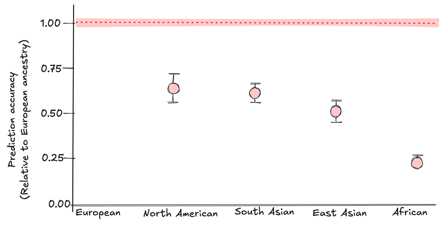
Redrawn from data reported in Martin AR, et al. Nature Genetics 51, 584–591 (2019). doi:10.1038/s41588-019-0379-x

The mechanism is in the recruitment, not the analysis. Allele frequencies and the patterns of correlation between nearby variants differ between populations; effect sizes estimated in one population do not transfer to another. No statistical method recovers ancestry that was never in the study. Closing the gap requires cohorts that include more populations.

Martin AR, et al. Clinical use of current polygenic risk scores may exacerbate health disparities. Nature Genetics 2019; 51(4): 584–591.

Underpowered studies an replicating results

A study can fail to replicate in an independent cohort for two different reasons: there is a genuine biological difference between the populations, or the original finding was not stable.

Module 2.2.1 established that underpowered studies not only miss true effects, they also detect signals that depend on which specific samples happened to be in the study. At low sample sizes, the detected features are partly determined by which individuals showed the strongest signal in that particular run. A different set of samples from the same population would produce a partly different result.

A study can fail to replicate in an independent cohort for two different reasons:

There is a genuine biological difference between the populations
The original finding was not stable.

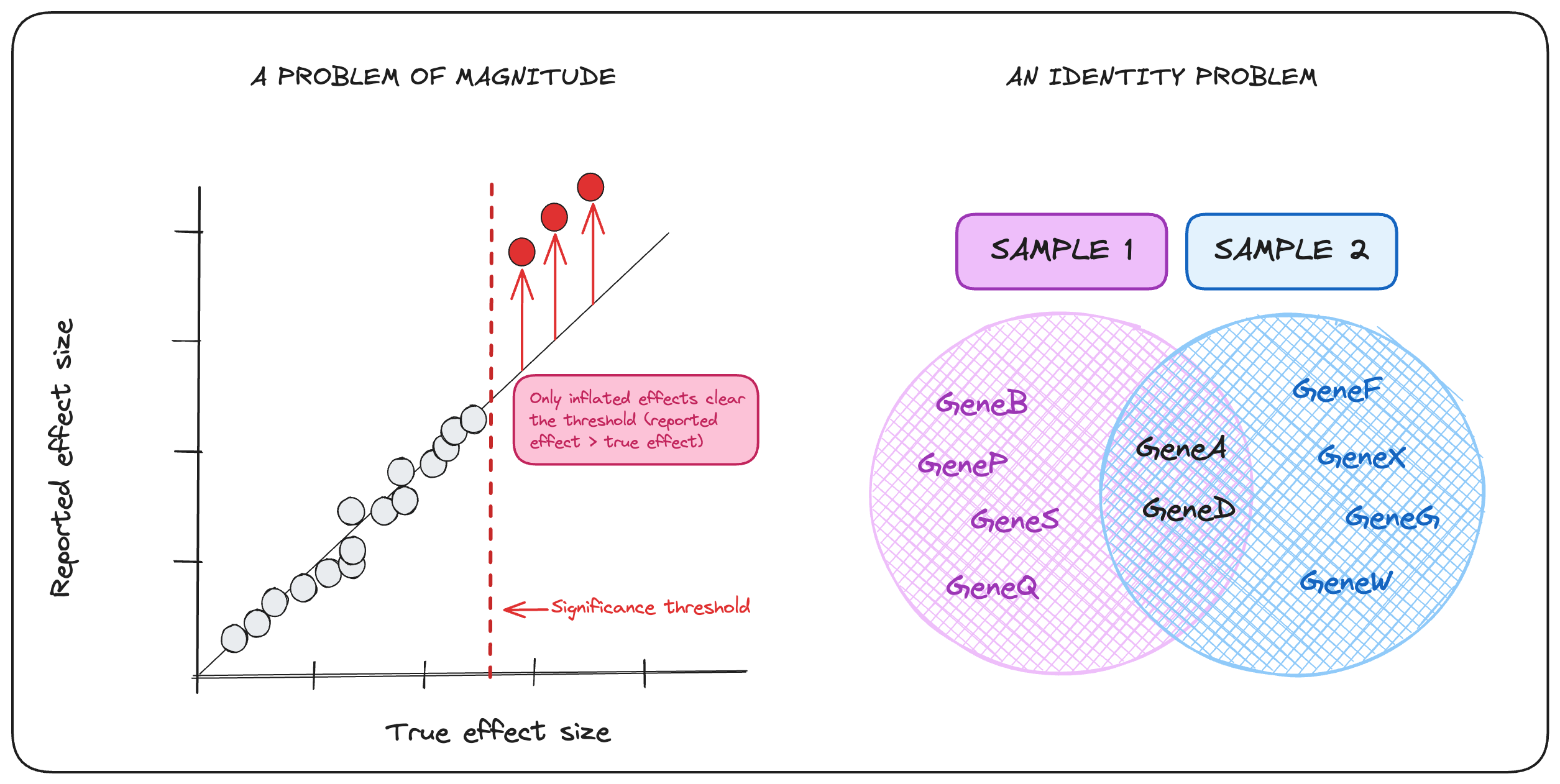
This is compounded by the winner's curse: in an underpowered study, the findings that do reach significance are those whose effect sizes were inflated by chance. The reported effect is therefore larger than the true underlying effect and a replication study, even an adequately powered one, will typically observe a smaller magnitude and may not replicate at all.

In transcriptomics, studies have shown that n = 3 per group detects between 20% and 40% of truly differential genes. The genes that appear in any given small study are an incomplete and variable subset of the true differential set. A list generated from n = 3 will overlap only partially with a list generated from a different set of n = 3 samples from the same population.

In metabolomics, a meta-analysis of 244 clinical studies found that 72% of statistically significant metabolites were reported in only one study. Each individual study detected a signal. Almost none detected the same one.

This is why power and generalisability are not entirely independent. When a finding fails to replicate in an independent cohort, the explanation could be a genuine population difference — or it could be that the original result was driven by sampling variation in an underpowered study. Without adequate power in the original study, distinguishing these two explanations is not straightforward.

Recommendations for follow-up

No single study can fully establish generalisability, and that is not the expectation. The table below describes three types of action. Each adds something, and they are not a checklist to complete before publication. The first costs nothing and can be done at the writing stage of any study. The second applies when design decisions are still open. The third is the most informative, but targeted approaches make it far more achievable than repeating the full study. Any one of these options strengthens a finding; none requires all three.

Action	What to do	What it addresses	Effort
State the limitation	In the results and conclusions, name the population (sex, age, species or strain, disease stage, recruitment setting), the tissue or sample type, the molecular layer, the platform, and the collection conditions. Do not claim past them. This requires that metadata was recorded. The checklist in Module 2.1.3 is what makes an honest scope statement possible.	Makes the scope of the finding explicit. Prevents overclaiming. Helps readers assess whether the finding applies to their own context.	Low. Done at the writing stage
Broaden the design	Recruit from additional sites, include both sexes, use multiple strains or varieties, or extend the time course. Each change widens the population the finding describes.	Directly expands who the finding applies to.	Medium to high. More biological variability means more samples needed (Module 2.2.1), more batch structure to manage (Module 2.1.2), and higher total cost (Module 2.2.2)
Validate using public datasets	Search existing reference repositories — TCGA (cancer genomics), UK Biobank (multi-omic population cohort), GTEx (multi-tissue transcriptomics), MetaboLights (metabolomics), PRIDE (proteomics) — for independent cohorts with different recruitment, protocols, and batch structure. A finding that replicates under different conditions is meaningful evidence of generalisability.	Tests whether the finding holds beyond the original study without collecting new samples.	Low to medium. Computation and analysis time, no new sample collection
Validate using targeted assays	Use the discovery study to identify a shortlist of candidates. Test those candidates in an independent cohort using lower-cost targeted assays — qPCR, ELISA, targeted mass spectrometry, or a targeted sequencing panel. This is faster and cheaper than re-running the full discovery protocol, and more informative about generalisability than a larger discovery study in the original cohort.	Confirms that key findings replicate in a different population using an independent approach.	Lower than full replication. Scales with the size of the candidate list

Activity: reading a cohort for scope

A research team publishes a plasma metabolomics study comparing people with type 2 diabetes (T2D) to normoglycaemic controls. The recorded metadata is:

Variable	Cases (n = 48)	Controls (n = 52)
Age (mean ± SD)	61 ± 8 years	60 ± 9 years
Sex	79% male	81% male
BMI (mean ± SD)	31.2 ± 4.1	28.6 ± 3.8
Recruitment	Single hospital diabetes outpatient clinic	Same hospital, GP referrals for metabolic screening
Disease duration	8–22 years (all established T2D)	—
Treatment	94% on metformin; 38% on additional glucose-lowering therapy	—
Collection	07:30–09:30, fasted ≥ 8 hours	Same
Platform	Untargeted LC-MS, positive and negative ion mode	—
Sample type	Plasma	Same

The study reports 34 metabolites significantly different between groups after FDR correction (the method for correcting for testing thousands of features simultaneously, covered in Module 2.2.1), including acylcarnitines, TCA cycle intermediates, and branched-chain amino acids.

Part 1: Who does this finding describe?

Using the metadata table above:

Which sex does the finding primarily describe, and why does this matter for metabolomics?
What disease stage and treatment context is described? Would you expect the same metabolite signature in newly diagnosed, untreated T2D?
What does the recruitment source suggest about the severity of T2D in the case group?
The collection protocol is tightly standardised (fasted, fixed time window). Is this a strength or a limitation for applying the result in other settings?

Part 2: What does the finding cover biologically?

The platform is untargeted LC-MS. Does this mean the study captured the complete metabolome?
The sample type is plasma. Does a difference in plasma metabolite concentrations establish that the same metabolites are altered inside the tissues where T2D pathology is primarily driven — liver and skeletal muscle?

Part 3: Recommendation

A follow-up study has budget for one of two designs: (a) the same design with n = 150 per group at the same single site, or (b) the same n = 48/52 split across two recruitment sites, with targeted validation of the 34 reported metabolites in matched skeletal muscle biopsies from a subset. Which do you recommend, and what specific limitation does each address?

Answer

Part 1

Approximately 80% of participants are male. Plasma metabolite concentrations differ systematically between sexes for acylcarnitines, amino acids, and lipid species — the classes reported in this study. The finding primarily describes T2D metabolite patterns in males. Whether the same signature appears in females is not answered by this study and cannot be inferred from it.
Cases have established T2D of 8–22 years duration; 94% are on metformin. Metformin directly alters mitochondrial function and gut microbiome composition, both of which affect acylcarnitine and amino acid profiles. The metabolite signature reflects T2D in a long-established, predominantly treated state. Whether the same signature appears in newly diagnosed, untreated T2D is a separate question. Some of the reported differences may reflect drug effects rather than disease biology.
A hospital diabetes outpatient clinic manages patients with more severe or complex T2D than those managed in primary care. The case group does not represent the full population of people with T2D — it represents those whose disease requires specialist management.
Standardised fasted collection at a fixed time window is a strength for internal consistency: it removes dietary state and circadian variation as sources of noise within the study, which helps detect genuine metabolite differences between groups. It is a limitation for applying the result in settings where standardised fasted collection is not feasible — which includes most clinical and field settings. A biomarker that requires fasted morning collection is only useful where that is possible.

Part 2

No. Untargeted LC-MS with positive and negative ion modes provides broad but incomplete coverage. Which metabolites are detected depends on their ionisation efficiency, the chromatographic method, the mass range scanned, and the spectral reference library used for identification. Many metabolite classes are poorly covered by standard LC-MS methods. The study reports differences among detectable metabolites, not across all metabolites.
No. Plasma metabolite concentrations reflect contributions from multiple organs simultaneously — liver, kidney, skeletal muscle, and others all secrete metabolites into circulation. An elevated plasma acylcarnitine concentration is consistent with reduced fatty acid oxidation but does not identify where in the body that reduction is occurring. Establishing that the same metabolites are altered within skeletal muscle tissue requires direct tissue measurement.

Part 3

Option (a) addresses the power and stability problem. At n ≈ 50 per group, the original study may have detected metabolites driven partly by sampling variation rather than a consistent biological signal. Increasing to n = 150 produces a more stable signature with fewer false positives and better coverage of smaller effects. It does not address sex imbalance, disease severity bias, treatment confounding, or the question of whether plasma differences reflect tissue-level changes.

Option (b) addresses generalisability directly. A second recruitment site tests whether the plasma signature holds in a different clinical population under different institutional conditions. Targeted validation in skeletal muscle tissue tests whether the plasma result reflects tissue-level pathology in the organ most relevant to T2D. The constraint is that at the original n, the discovery signature being validated may itself be unstable.

The right choice depends on the primary aim. If the goal is a stable, reliable plasma biomarker — something deployable in clinical practice — option (a) is the necessary first step: validating an unstable list in a second cohort provides limited information. If the goal is biological understanding of T2D pathology in muscle, option (b) addresses that directly. In either case, the reported findings should explicitly state who they describe and what they do not cover.

Module 2.3.1 takeaways

Generalisability has two components: population generalisability and biological scope.
Internal validity and external validity are independent. Controlling confounding does not widen the population the finding describes.
Each molecular layer has different scope constraints.
Narrowing a cohort can improve power and interpretability. Broadening a cohort can improve generalisability. These trade-offs are governed by the same constraints as sample size and batch management.
Underpowered studies produce findings that may not replicate in independent cohorts even within the same population, because the detected features depend partly on which samples happened to be included.
Always state the scope of your finding explicitly: the population, tissue, molecular layer, platform, and collection conditions.
External validation does not require repeating the full study. Public datasets and targeted low-cost assays in a second cohort both provide evidence of generalisability at lower cost than a full replication.